Simulating Emotions during a Basketball Game - Just a Feeling in the Crowd
Sporting events host witness to a wide range of human emotion. The emotional ups and downs are especially clear among invested fans. Fans experience the joy and excitement of a triumphant comeback, or the anxiety and disappointment of a loss. It is particularly interesting to see how emotions differ from two opposing fan groups watching the same match.
I decided to perform some simulations on how a crowd of fans would react during a basketball game. Why basketball? Two reasons: First is the frequency of scoring (more baskets = more reactive simulation), and second is that the NBA finals are in swing at time of writing.
Below I’ve described the parameters of the simulation in detail and provided reproducible code for all examples, but here’s the quick and dirty. I’m simulating fans’ happiness and nerves (valence and arousal). Happiness reflects baskets scored (up for team basket and down for enemy basket) and overall team performance. Nerves reflects baskets scored, time remaining in game, and the difference between score (higher for closer game). There are other parameters involved that are described in more detail below.
Let’s run the simulation! I’m simulating a short game that’s about 16 minutes long, but the simulation is sped up. There are 25 fans per team with each dot representing a fan. Blue dots root for the blue team and red dots for red. In this game, blue starts ahead, but red makes a rallying comeback.
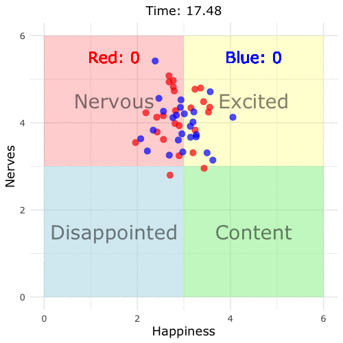
What are we seeing here? As the game progresses, fans move into different emotional states. I’ve used the terms content, disappointed, nervous, and excited as helpful placeholders, but we should think of these in terms of varying along dimensions of valence (e.g., happiness) and arousal (e.g., nerves, excitedness). For example, when their team is doing well, fans are happier, but they’re only excited when the score is close. For each basket, there’s a brief spike in arousal and happiness. As the game draws closer to an end, fans get more excited/anxious, especially if the score is close.
So how would this play out if one team decimated the other? Let’s give the red team a slight edge over blue:
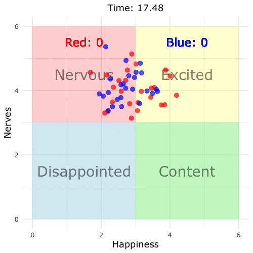
Notice how ‘excited’ becomes ‘content’ and ‘nervous’ turns to ‘disappointment’ because the difference becomes insurmountable for the blue team. We can plug in any numbers for this function to produce different results. However, the algorithm is highly sensitive to small changes in scoring chance because this is calculated for every second of the game.
Going Behind the Simulation
Skip this if you have no interest in the psychology of emotions. What I’m striving to simulate are the laws of emotion dynamics (Kuppens & Verduyn, 2017). Emotions change from moment to moment, but there’s also some stability from one moment to the next. Apart from when a basket is scored, most fans cluster around a particular state (this is called an attractor state). Any change is attributable to random fluctuations (e.g., one fan spills some of their beer, maybe another fan sees an amusing picture of a cat on their phone). When a basket is scored, this causes a temporary fluctuation away from the attractor state, after which people resort back to their attractor. More gradual situational factors result in small changes in attractors too. This is why arousal tends to increase with closer games and when the game is approaching the end.
Detailed Aspects of Simulation and Code
There are two parts to this simulation. Part 1 simulates a basketball game for a specified duration of time (n_seconds) and specified probabilities of scoring. The simulation is also designed with a small post game period - sort of like a cool down after the game. During the post game, fans’ arousal returns to baseline.
The second and more complicated part of the simulation is the emotional part. Each fan has a score on valence and arousal at each second. These can be further broken down into fixed effects and random effects. The fixed effect for valence is described as follows:
\[Valence = 3 + \beta_{1overall.difference}(.20) + \beta_{2recent.score(1.5 + \frac{current.time}{total.time})} - \beta_{3recent.enemy.score}\]
The fixed effect for arousal looks like this:
\[Arousal = 3 + \beta_{1 (\frac{current.time}{total.time})(.75)(post.game)} + \beta_{2(1 - \sqrt{|difference|})} + \beta_{3|recent.basket|}\]
The exact values for these coefficients are somewhat arbitrary. They resulted from a lot of trial and error to identify which best simulated emotion dynamics.
Each fan’s valence and arousal is calculated using the above equations + variability. The variability is added by applying random variation to the first constant in the above equations and white noise with a simulated ARIMA model. On top of this, I used a kernel regression smoother to smooth out each fan’s trajectory. To simulate delayed reaction time to baskets, I added some lags at random intervals - otherwise the simulated fans appear to react quicker than the score board. Here’s what all of this looks like for one fan’s valence over time:
library(tidyverse)

game_long %>%
  filter(fan == 1,
         team == "team1") %>%
  ggplot(aes(x = second, y = valence)) +
  geom_line(color = "red", size = 1) +
  theme_minimal(base_size = 16) +
  labs(title = "Fan One's Valence over Time",
       x = "Time",
       y = "Valence") +
  theme(legend.position = "none",
        axis.title.x = element_text(size = 18),
        axis.title.y = element_text(size = 18),
        plot.title = element_text(size = 18, hjust = .5))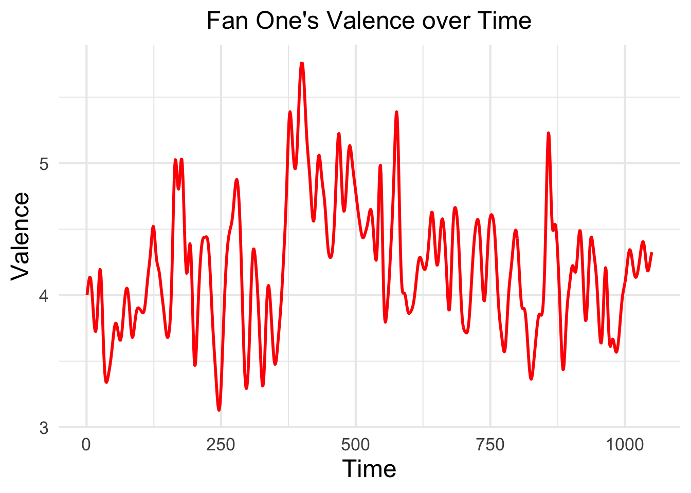
We can see this across all fans as well:
game_long %>%
  ggplot(aes(x = instance, color = team)) +
  geom_line(aes(y = valence), alpha = .65) +
  labs(title = "Valence over Time",
       x = "Time",
       y = "Valence") +
  theme_minimal() +
  theme(legend.position = "none",
        axis.title.x = element_text(size = 18),
        axis.title.y = element_text(size = 18),
        plot.title = element_text(size = 18, hjust = .5))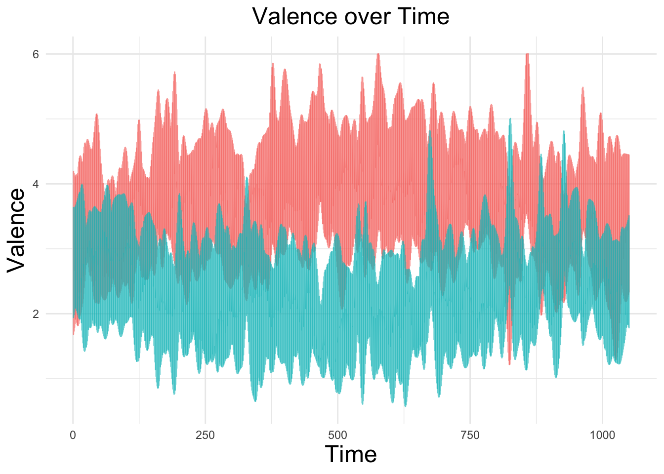
And for arousal…
game_long %>%
  ggplot(aes(x = instance, color = team)) +
  geom_line(aes(y = arousal), alpha = .65) +
  labs(title = "Arousal over Time",
       x = "Time",
       y = "Arousal") +
  theme_minimal() +
  theme(legend.position = "none",
        axis.title.x = element_text(size = 18),
        axis.title.y = element_text(size = 18),
        plot.title = element_text(size = 18, hjust = .5))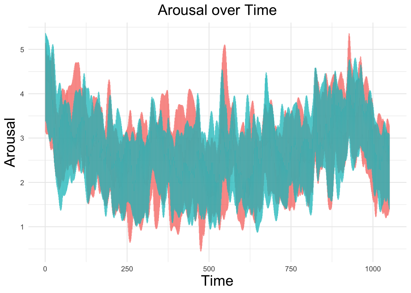
For those interested, here’s the full code for the simulation and first animation. Have fun with it! I’m also looking for ways to improve it. Ironically, I don’t watch a ton of sports, so if you think I’m open to input on how to make it more realistic!
library(tidyverse)
library(forecast)
library(gganimate)
library(extrafont)

game_simulation <- function(n_seconds = 1000, n_fans = 25, team1_prob = 0.012, team2_prob = 0.012) {

  score_board <- data.frame(matrix(nrow = n_seconds, ncol = 5))
  colnames(score_board) <- c("second", "team1_score", "team2_score", "difference", "end_game")
  score_board$second <- c(1:n_seconds)

  score_board$team1_score <- cumsum(sample(c(0, 1, 1.5), n_seconds, replace = TRUE, prob = c(1 - team1_prob, team1_prob * .90, team1_prob * .10)))

  score_board$team2_score <- cumsum(sample(c(0, 1, 1.5), n_seconds, replace = TRUE, prob = c(1 - team2_prob, team2_prob * .90, team2_prob * .10)))

  score_board$difference <- score_board$team1_score - score_board$team2_score

  score_board$end_game = 1

  total_time <- n_seconds + n_seconds * .05

  end_time <- data.frame(max(score_board$second + 1):(total_time))
  colnames(end_time) <- "second"
  end_state <- score_board[nrow(score_board), 2:5]
  post_game <- data.frame(matrix(nrow = n_seconds * .05, ncol = 0),
                          "team1_score" = end_state$team1_score,
                          "team2_score" = end_state$team2_score,
                          "difference" = end_state$difference,
                          "end_game" = 0)

  post_game <- cbind(end_time, post_game)

  score_board <- rbind(score_board, post_game)

  valence <- function(time, overall_difference, recent_team_score, recent_enemy_score) (
    (overall_difference * .20) + (recent_team_score * (1.5 + time/length(time))) - (recent_enemy_score)
  )

  arousal <- function(time, difference, recent_score, end_game) (
    ((time/n_seconds) * .75 * end_game) + (1 - sqrt(abs(difference))) + abs(recent_score * 1.5)
  )

  team1_valence <- data.frame(matrix(nrow = total_time, ncol = 0))
  team1_arousal <- data.frame(matrix(nrow = total_time, ncol = 0))
  team2_valence <- data.frame(matrix(nrow = total_time, ncol = 0))
  team2_arousal <- data.frame(matrix(nrow = total_time, ncol = 0))

  for(i in 1:n_fans) {

    team1_valence[[i]] <- ksmooth(x = score_board$second,
                                  y = rnorm(n = 1, mean = 3, sd = .25) + (arima.sim(list(order = c(1, 0, 1), ma = -.1, ar = c(.9)), n = total_time) * .25) + valence(time = score_board$second,
                                  overall_difference = score_board$difference,
                                  recent_team_score = lag(score_board$team1_score, n = sample(c(1:5), 1), default = 0) - lag(score_board$team1_score, n = sample(c(6:8), 1), default = 0),
                                  recent_enemy_score = lag(score_board$team2_score, n = sample(c(1:5), 1), default = 0) - lag(score_board$team2_score, n = sample(c(6:8), 1), default = 0)),
                                  bandwidth = total_time/100, kernel = "normal")$y

  }

  colnames(team1_valence) <- paste0("team1_", "valence_", 1:n_fans)
  team1_valence[team1_valence > 6] <- 6
  team1_valence[team1_valence < 0] <- 0

  for(i in 1:n_fans) {
    team1_arousal[[i]] <- ksmooth(x = score_board$second,
                                  y = rnorm(n = 1, mean = 3, sd = .25) + (arima.sim(list(order = c(1, 0, 1), ma = -.1, ar = c(.9)), n = total_time) * .25) + arousal(time = score_board$second,
                                  difference = score_board$difference,
                                  recent_score = lag(score_board$difference, n = sample(c(1:3), 1), default = 0) - lag(score_board$difference, n = sample(c(4:6), 1), default = 0),
                                  end_game = score_board$end_game),
                                  bandwidth = total_time/100, kernel = "normal")$y
  }

  colnames(team1_arousal) <- paste0("team1_", "arousal_", 1:n_fans)

  team1_arousal[team1_arousal > 6] <- 6
  team1_arousal[team1_arousal < 0] <- 0

  for(i in 1:n_fans) {
    team2_valence[[i]] <- ksmooth(x = score_board$second,
                                  y = rnorm(n = 1, mean = 3, sd = .25) + (arima.sim(list(order = c(1, 0, 1), ma = -.1, ar = c(.9)), n = total_time) * .25) + valence(time = score_board$second,
                                  overall_difference = -score_board$difference,
                                  recent_team_score = lag(score_board$team2_score, n = sample(c(1:5), 1), default = 0) - lag(score_board$team2_score, n = sample(c(6:8), 1), default = 0),
                                  recent_enemy_score = lag(score_board$team1_score, n = sample(c(1:5), 1), default = 0) - lag(score_board$team1_score, n = sample(c(6:8), 1), default = 0)),
                                  bandwidth = total_time/100, kernel = "normal")$y
  }

  colnames(team2_valence) <- paste0("team2_", "valence_", 1:n_fans)

  team2_valence[team2_valence > 6] <- 6
  team2_valence[team2_valence < 0] <- 0

  for (i in 1:n_fans) {
    team2_arousal[[i]] <- ksmooth(x = score_board$second,
                                  y = rnorm(n = 1, mean = 3, sd = .25) + (arima.sim(list(order = c(1, 0, 1), ma = -.1, ar = c(.9)), n = total_time) * .25) + arousal(time = score_board$second,
                                  difference = score_board$difference,
                                  recent_score = lag(score_board$difference, n = sample(c(1:3), 1), default = 0) - lag(score_board$difference, n = sample(c(4:6), 1), default = 0),
                                  end_game = score_board$end_game),
                                  bandwidth = total_time/100, kernel = "normal")$y
  }

  colnames(team2_arousal) <- paste0("team2_", "arousal_", 1:n_fans)

  team2_arousal[team2_arousal > 6] <- 6
  team2_arousal[team2_arousal < 0] <- 0

  game_affect <- cbind(score_board, team1_valence, team1_arousal, team2_valence, team2_arousal)

  return(game_affect)
}

set.seed(060519)

game <- game_simulation(n_seconds = 1000, n_fans = 25)

game_long <- game %>%
  mutate(instance = row_number(),
         team1_score = team1_score * 2,
         team2_score = team2_score * 2) %>%
  select(instance, everything()) %>%
  select(-end_game) %>%
  gather(key = "team", value = "score", c(team1_valence_1:length(game))) %>%
  separate(col = team, into = c("team", "dimension", "fan"), sep = "_") %>%
  spread(dimension, score)

p <- game_long %>%
  ggplot() +
  annotate("rect", xmin = 0, xmax = 3, ymin = 0, ymax = 3, alpha = 0.5, fill = "lightblue") +
  annotate("rect", xmin = 3, xmax = 6, ymin = 0, ymax = 3, alpha = 0.5, fill = "lightgreen") +
  annotate("rect", xmin = 0, xmax = 3, ymin = 3, ymax = 6, alpha = 0.2, fill = "red") +
  annotate("rect", xmin = 3, xmax = 6, ymin = 3, ymax = 6, alpha = 0.2, fill = "yellow") +
  annotate("text", x = c(1.5, 4.5, 1.5, 4.5), y = c(1.5, 1.5, 4.5, 4.5), label = c("Disappointed", "Content", "Nervous", "Excited"),
           size = 10, alpha = .50, family = "Verdana") +
  geom_text(aes(x = 1.5, y = 5.5, label = paste("Red:", team1_score)), size = 8, color = "red", family = "Verdana") +
  geom_text(aes(x = 4.5, y = 5.5, label = paste("Blue:", team2_score)), size = 8, color = "blue", family = "Verdana") +
  geom_point(aes(x = valence, y = arousal, color = team), alpha = .70, size = 4) +
  scale_x_continuous(limits = c(0, 6)) +
  scale_y_continuous(limits = c(0, 6)) +
  scale_color_manual(values = c("red", "blue")) +
  labs(title = 'Time: {round((max(game_long$second) - frame_time)/60, 2)}',
       x = "Happiness",
       y = "Nerves") +
  theme_minimal(base_size = 16) +
  transition_time(second) +
  theme(legend.position = "none",
        axis.title.x = element_text(size = 18),
        axis.title.y = element_text(size = 18),
        plot.title = element_text(size = 18, hjust = .5),
        text = element_text(family = "Verdana"))

game1 <- animate(p, nframes = 1062, width = 500, height = 500, fps = 10, end_pause = 12)

game1
References
Kuppens P, Verduyn P. (2017). Emotion dynamics. Current Opinion in Psychology. 17, 22–26. doi: 10.1016/j.copsyc.2017.06.004.