An Intuitive Look at Binomial Probability in a Bayesian Context
Binomial probability is the relatively simple case of estimating the proportion of successes in a series of yes/no trials. The perennial example is estimating the proportion of heads in a series of coin flips where each trial is independent and has possibility of heads or tails. Because of its relative simplicity, the binomial case is a great place to start when learning about Bayesian analysis. In this post, I will provide a gentle introduction to Bayesian analysis using binomial probability as an example. Instead of coin flips, we’ll imagine a scenario where we are mining for gold!
Setting the Scene
There’s talk in the town that gold is to be found in the nearby hills! We focus on a local merchant who buys gold from prospectors to trade with neighbouring towns. The merchant needs to know how much gold is out there so that they can set a competitive price for buying and selling. The merchant decides to investigate the proportion of gold in the hills by collecting data. It is impossible to survey the entire landscape, but the merchant assumes that a sample of the hills will provide a good estimate of the total proportion of gold.
The merchant’s goal is to estimate the true proportion of gold in the hills. We will use \(\theta\) to represent this quantity that we are trying to estimate.
Simulating the Problem
For this example, we will simulate the entire landscape as a 100 x 100 grid. We will allow each of the 10,000 points on the grid to have a probability of .10 (10%) of containing gold. This is our chosen value of \(\theta\) for the simulation. We’ll also identify a sample 10 x 10 grid. Here’s a plot of the simulated landscape identifying the location of gold and the sample area.
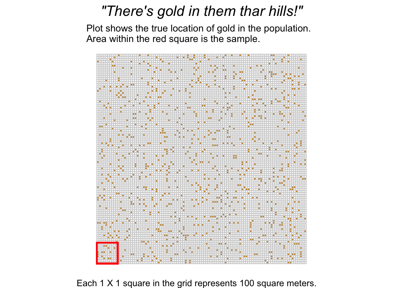
Remember we are omniscient but our merchant knows nothing about where the gold is and how much there truly is. Bayesian statistics is all about dealing with uncertainty by incorporating information from new data and prior sources of information.
Bayes’ Theorem
I’m sure that most readers have encountered Bayes’ theorem at some point in their stats journey, although maybe the notation was different. We are most interested in computing the posterior probability, which we denote as \(p(\theta|y)\). It combines information obtained from the data \(y\) and our prior information (what we already know about \(\theta\)). Expressed more formally,
\[p(\theta|y)=\frac{p(y|\theta)p(\theta)}{p(y)}\]
where \(\theta\) (\(p(\theta|y)\) is the posterior probability; \(p(y|\theta)\) is the data-generating process, usually referred to as the likelihood; \(p(\theta)\) is the prior probability of \(\theta\); and \(p(y)\) is a normalizing constant. We won’t worry ourselves with the normalizing constant, \(p(y)\) as it doesn’t affect our conclusions. Thus, we’ll stick with the nonnormalized posterior likelihood:
\[p(\theta|y)=p(y|\theta)p(\theta)\]
At first, this formula can be quite confusing. When I first encountered it, I was confused by what \(\theta\) represented (and this stemmed from a fuzzy understanding of likelihood estimation I had at the time). What’s important to understand is that \(\theta\) is an unknown parameter, but in order to estimate our uncertainty about \(\theta\) we are going to try out different values of \(\theta\).
For example, we want to know the proportion of gold in the area which ranges from 0 to 1 (0 being no gold; 1 being all gold). So in our equation, \(\theta\) would represent all values between 0 and 1. However, there are infinite values between 0 and 1, so in practice we could try out values between 0 and 1. In this example, we will use a relatively simple process called grid approximation where we use an equally spaced grid of values between 0 and 1 for \(\theta\).
Binomial Likelihood
Let’s tackle the first piece of Bayes’ theorem: the likelihood, \(p(y|\theta)\). Here, we are essentially asking the question: “how likely is the data, given a particular value for \(\theta\)?” Here, we introduce the binomial likelihood function:
\[p(y|\theta)=\theta^y(1-\theta)^{n-y}\]
where \(y\) is the number of successes and \(n\) is the number of trials.
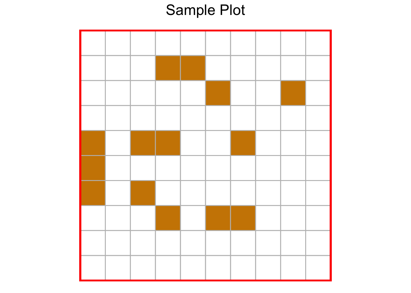
Let’s return to our gold merchant and see how we can express the likelihood in terms of the data the merchant observes. Imagine our merchant collects data by digging each of the 10 x 10 squares in the sample. The merchant finds that 14 out of 100 spaces in the sample contain gold:
Here’s how we express the data in terms of the binomial likelihood function:
\[p(y|\theta)=\theta^{14}(1-\theta)^{100-14}\]
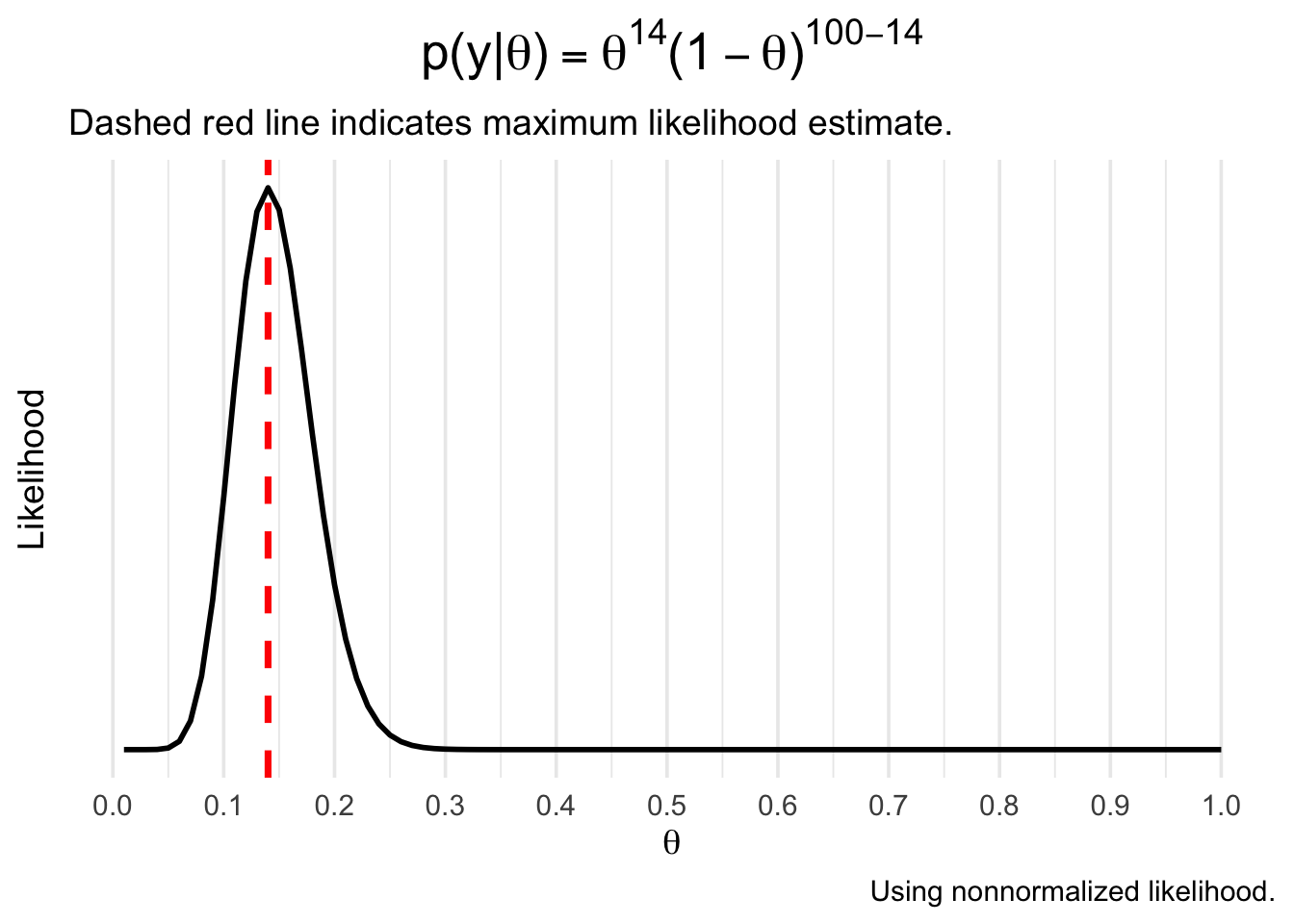
If we compute \(p(y|\theta)\) across the grid of \(\theta\) values from 0 to 1, we get the following probability density:
Reproducing this in R is fairly simple - we could substitute the values into the binomial formula, or just use the built-in dbinom function. We then create a dataframe containing the likelihood for each theta and use ggplot2 from the tidyverse to draw the plot:
library(tidyverse)

# use seq(.01, 1, .01) to generate a sequence from .01 to 1 in .01 increments
likelihood <- dbinom(x = 14, size = 100, prob = seq(.01, 1, .01))

# creating a data frame with 'likelihood' for plotting
df <- data.frame(theta = seq(.01, 1, .01),
                 likelihood)

# create the plot
ggplot(df, aes(x = theta, y = likelihood)) +
  geom_line(size = 1) +
  labs(x = TeX("$\\theta$"),
       y = "Likelihood",
       title = TeX("$p(y|\\theta) = \\theta^{14}(1 - \\theta)^{100 - 14}$"),
       subtitle = "Dashed red line indicates maximum likelihood estimate.",
       caption = "Using nonnormalized likelihood.") +
  geom_vline(xintercept = .14, size = 1.25, color = "red", linetype = 2) +
  scale_x_continuous(breaks = seq(0, 1, by = .10)) +
  theme_minimal(base_size = 14) +
  theme(axis.text.y = element_blank(),
        axis.ticks.y = element_blank(),
        panel.grid.major.y = element_blank(),
        panel.grid.minor.y = element_blank(),
        plot.title = element_text(hjust = .5, size = 20))
Not surprisingly, the most likely value of \(\theta\) (the maximum likelihood estimate) is .14. In Bayesian statistics, however, we aren’t content with just the point estimate and instead we use the entire density to express uncertainty about \(\theta\).
Incorporating Prior Information
Imagine that our merchant hears rumours that each 100 square meters of land has a 20% probability of containing gold. We now want to incorporate this prior information into our model. \(p(\theta)\) is the prior probability of \(\theta\) and it can represent past data or even subjective knowledge about the likely value and uncertainty of \(\theta\).
A common approach when choosing priors is to identify a conjugate prior: a formula for expressing the prior that has a similar data structure to that of the likelihood. In this case, a conjugate prior for the binomial likelihood is the beta function:
\[\text{beta}(a,b)=\theta^{a-1}(1-\theta)^{b-1}\]
where \(a\) can represent successes and \(b\) can represent failures.
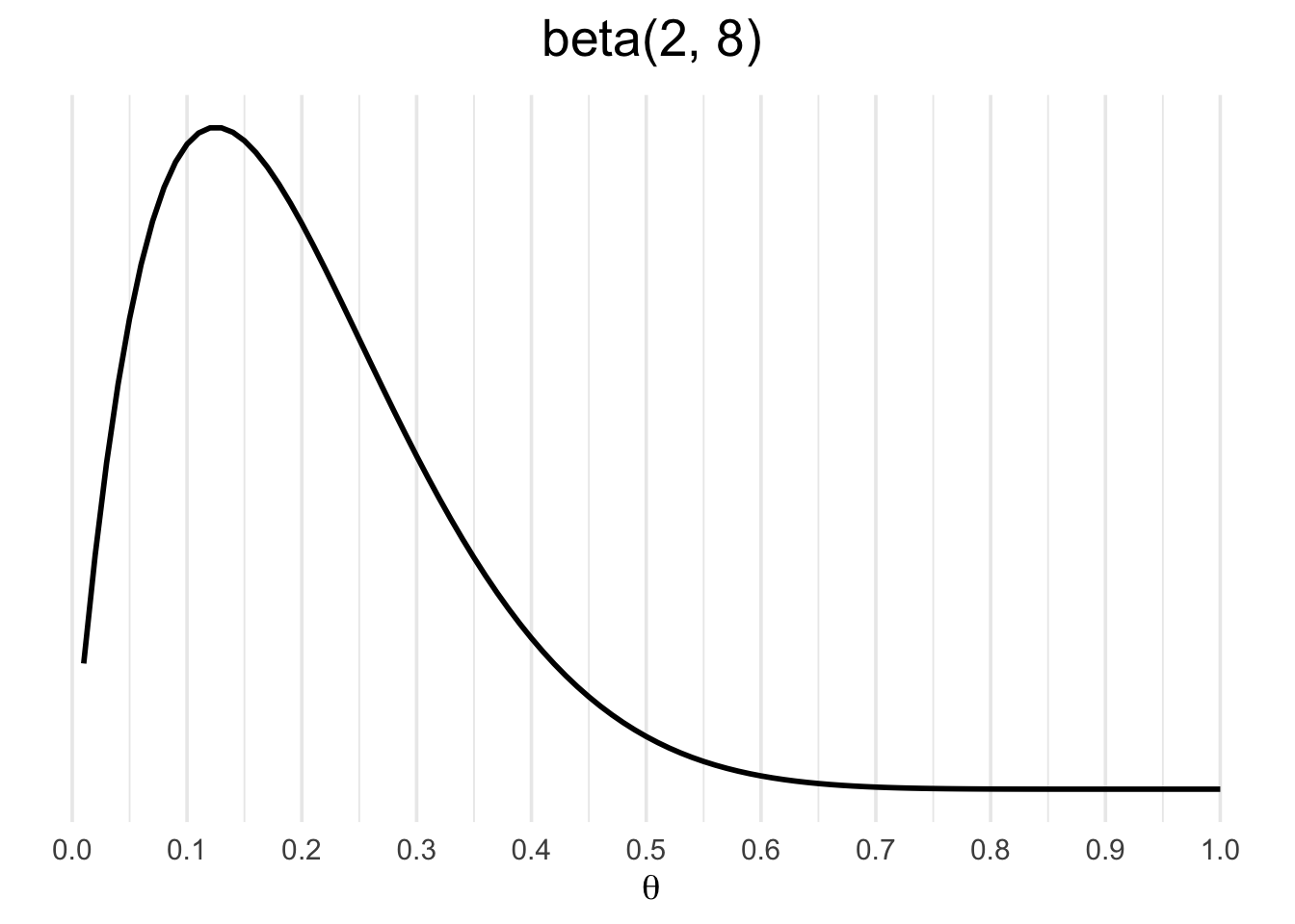
Notice the similarity between the formulas for the binomial and beta functions. They have identical data structures, which makes the beta a conjugate prior for the binomial likelihood. Let’s use a \(\text{beta}(2,8)\) as a prior, representing our knowledge of a rumored 20% probability of gold.
Similarly, you can reproduce this using the dbeta function in R:
# here we use x as a sequence from .01-1
b_likelihood <- dbeta(x = seq(.01, 1, .01), shape1 = 2, shape2 = 8)

df <- data.frame(theta = seq(.01, 1, .01),
                 b_likelihood)

df %>%
  ggplot(aes(x = theta, y = b_likelihood)) +
  geom_line(size = 1) +
  labs(x = TeX("$\\theta$"),
       y = NULL,
       title = TeX("beta(2,8)")) +
  scale_x_continuous(breaks = seq(0, 1, by = .10)) +
  theme_minimal(base_size = 14) +
  theme(axis.text.y = element_blank(),
        axis.ticks.y = element_blank(),
        panel.grid.major.y = element_blank(),
        panel.grid.minor.y = element_blank(),
        plot.title = element_text(hjust = .5, size = 20))
Why use a beta prior instead of another binomial density? The reason is that the binomial density is dependent on a sample size parameter n, whereas the beta density is not. It is more convenient to express our prior knowledge without n.
Getting the Posterior
The posterior probability, \(p(\theta|y)\) takes into account the data and the prior. It is often viewed as a compromise between the data likelihood and the prior probability. This is more easily understood graphically:
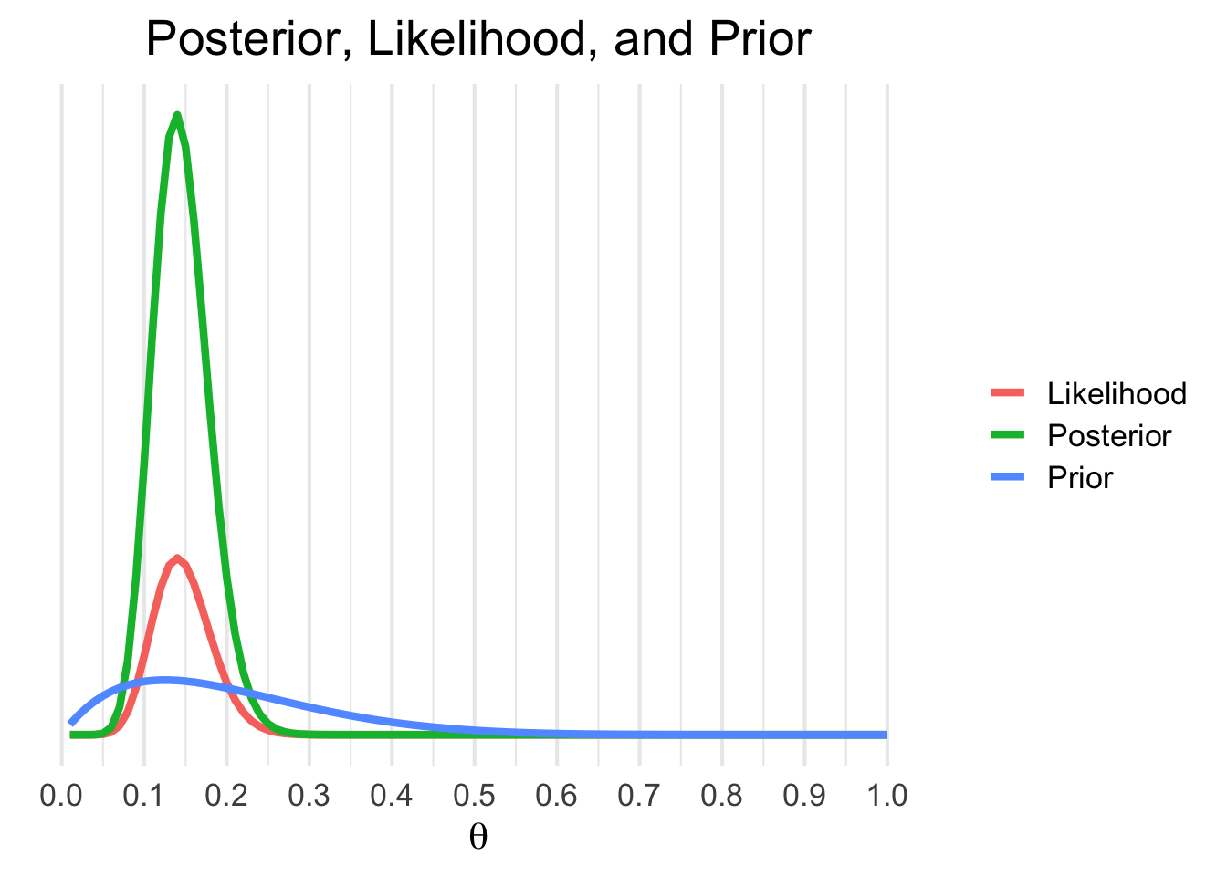
Here’s how to produce this figure:
theta <- seq(.01, 1, .01)
prior <- dbeta(x = theta, shape1 = 2, shape2 = 8)

#multiply the binomial likelihood by 100 to express it in 'probability terms' like the beta
likelihood <- dbinom(x = 14, size = 100, prob = theta) * 100
posterior_density <- likelihood * prior

df <- data.frame(theta = theta,
                 likelihood = likelihood,
                 prior = prior,
                 pd = posterior_density)

# use pivot_longer to create a variable out of likelihood vs. prior vs. posterior
data_long <- pivot_longer(df, cols = c(likelihood, prior, pd))

data_long %>%
  ggplot(aes(x = theta, y = value, color = name)) +
  geom_line(size = 1.5) +
  labs(x = TeX("$\\theta$"),
       y = NULL,
       color = NULL,
       title = "Posterior, Likelihood, and Prior") +
  scale_color_discrete(labels = c("Likelihood", "Posterior", "Prior")) +
  scale_x_continuous(breaks = seq(0, 1, by = .10)) +
  theme_minimal(base_size = 16) +
  theme(axis.text.y = element_blank(),
        axis.ticks.y = element_blank(),
        panel.grid.major.y = element_blank(),
        panel.grid.minor.y = element_blank(),
        plot.title = element_text(hjust = .5, size = 20))
The above chart shows the posterior, likelihood, and prior side by side. Notice how the prior (in blue) contains less certainty than the likelihood. The posterior density is simply the prior multiplied by the likelihood, thus it contains information from both sources. It’s a general rule that in instances when there is a lot of data and our prior is mostly uninformative that the likelihood will overwhelm the prior.
If we were to extend this further to make actual conclusions about our uncertainty of the proportion of gold in the hills, we would need to draw random samples from the posterior distribution and generate interval estimates based on these draws. For this post, however, we will stick to a graphical evaluation of \(p(\theta|y)\).
An Animated Example
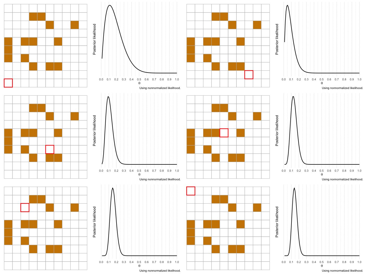
I’m a huge proponent of using animations to illustrate complicated topics (if you haven’t yet, you should consider watching 3Blue1Brown’s videos covering mathematics concepts). So I want to end by bringing to life our example of a gold miner estimating the proportion of gold in a section of land. We’ll use the same information as before, but the difference this time is that the gold miner will investigate each 1 x 1 section of land at a time and update the likelihood.
The animation begins with our merchant-miner (indicated by the red square) on square 1,1. As the merchant covers the sample, the influence of the likelihood over the prior increases and there is more certainty in the estimate. If we expanded our sample to cover more of the territory, our estimate would get even closer to the true value of \(\theta\) and we’d be more certain about it.
Conclusions
The binomial likelihood serves as a great introductory case into Bayesian statistics. It may seem like overkill to use a Bayesian approach to estimate a binomial proportion, indeed the point estimate equals the sample proportion. But remember that it’s far more important to get an estimate of uncertainty as opposed to a simple point estimate.
There’s a lot we didn’t cover here; namely, making inferences from the posterior distribution, which typically involves sampling from the posterior distribution. As well, I hope to soon extend into more practical cases such as logistic regression, mixture modeling, etc, with demonstrations using Stan.
If you’re eager for more examples and tutorials with Bayesian statistics, I’d recommend watching this video series by Rasmus Bååth. John Kruschke’s book Doing Bayesian Data Analysis is a great introductory text. If you’re up for the challenge, consider also Bayesian Data Analysis, 3rd edition by Gelman et al, widely considered to be the Bayesian Bible. Much of the content for this blog post was inspired from the first few chapters of that book.