A Model and Simulation of Emotion Dynamics
Emotion dynamics is the study of how emotions change over time. Sometimes our feelings are quite stable, but other times capricious. Measuring and predicting these patterns for different people is somewhat of a Holy Grail for emotion researchers. In particular, some researchers are aspiring to discover mathematical laws that capture the complexity of our inner emotional experiences - much like physicists divining the laws that govern objects in the natural environment. These discoveries would revolutionize our understanding of our everyday feelings and when our emotions can go awry.
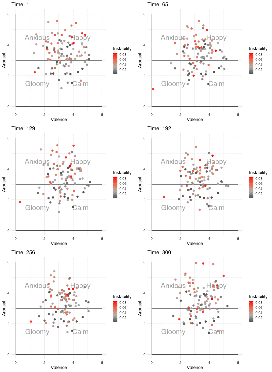
This series of blog posts, which I kicked off earlier this month with a simulation of emotions during basketball games, is inspired by researchers like Peter Kuppens and Tom Hollenstein (to name a few) who have collected and analyzed reams of intensive self-reports on people’s feelings from one moment to the next. My approach is to reverse engineer these insights and generate models that simulate emotions evolving over time - like this:
Affective State Space
We start with the affective state space - the theoretical landscape on which our conscious feelings roam free. This space is represented as two-dimensional, although we acknowledge that this fails to capture all aspects of conscious feeling. The first dimension, represented along the x-axis, is valence and this refers to how unpleasant vs. pleasant we feel. The second dimension, represented along the y-axis, is arousal. Somewhat less intuitive, arousal refers to how deactivated/sluggish/sleepy vs. activated/energized/awake we feel. At any time, our emotional state can be defined in terms of valence and arousal. So if you’re feeling stressed you would be low in valence and high in arousal. Let’s say you’re serene and calm, then you would be high in valence and low in arousal. Most of the time, we feel moderately high valence and moderate arousal (i.e., content), but if you’re the type of person who is chronically stressed, this would be different.
This is all well and good when we think about how we’re feeling right now, but it’s also worth considering how our emotions are changing. On a regular day, our emotions undergo minor fluctuations - sometimes in response to minor hassles or victories, and sometimes for no discernible reason. In this small paragraph, I’ve laid out a number of parameters, all of which vary between different people:
- Attractor: Our typical emotional state. At any given moment, our feelings are pulled toward this state. Some people tend to be happier, whereas others are less happy.
- Stability: How emotionally stable one is. Some people are more emotionally stable than others. Even in the face of adversity, an emotionally stable person keeps their cool.
- Dispersion: The range of our emotional landscape. Some people experience intense highs and lows, whereas others persist somewhere in the middle.
We’ll keep all of this in mind for the simulation. We’ll start with a fairly simple simulation with 100 hypothetical people. We’ll need the following packages.
library(psych)
library(tidyverse)
library(sn)
And then we’ll create a function that performs the simulation. Note that each person i has their own attractor, recovery rate, stability, and dispersion. For now we’ll just model random fluctuations in emotions, a sort of Brownian motion. You can imagine our little simulatons (fun name for the hypothetical people in the simulation) sitting around on an average day doing nothing in particular.
simulate_affect <- function(n = 2, time = 250, negative_event_time = NULL) {
  dt <- data.frame(matrix(nrow = time, ncol = 1))
  colnames(dt) <- "time"
  dt$time <- 1:time

  valence <- data.frame(matrix(nrow = time, ncol = 0))
  arousal <- data.frame(matrix(nrow = time, ncol = 0))

  for(i in 1:n) {
    attractor_v <- rnorm(1, mean = 3.35, sd = .75)
    instability_v <- sample(3:12, 1, replace = TRUE, prob = c(.18, .22, .18, .15, .8, .6, .5, .4, .2, .1))
    dispersion_v <- abs(rsn(1, xi = .15, omega = .02, alpha = -6) * instability_v) #rsn simulates a skewed distribution.
    if(!is.null(negative_event_time)) {
      recovery_rate <- sample(1:50, 1, replace = TRUE) + negative_event_time
      negative_event <- (dt$time %in% negative_event_time:recovery_rate) * seq.int(50, 1, -1)
    }
    else {
      negative_event <- 0
    }
    valence[[i]] <- ksmooth(x = dt$time,
                            y = (negative_event * -.10) + arima.sim(list(order = c(1, 0, 0),
                                               ar = .50),
                                          n = time),
                            bandwidth = time/instability_v, kernel = "normal")$y * dispersion_v + attractor_v

#instability is modelled in the bandwidth term of ksmooth, such that higher instability results in higher bandwidth (greater fluctuation).
#dispersion scales the white noise (arima) parameter, such that there are higher peaks and troughs at higher dispersion.

    attractor_a <- rnorm(1, mean = .50, sd = .75) + sqrt(instability_v) #arousal attractor is dependent on instability. This is because high instability is associated with higher arousal states.
    instability_a <- instability_v + sample(-1:1, 1, replace = TRUE)
    dispersion_a <- abs(rsn(1, xi = .15, omega = .02, alpha = -6) * instability_a)
    arousal[[i]] <- ksmooth(x = dt$time,
                            y = (negative_event * .075) + arima.sim(list(order = c(1, 0, 0),
                                               ar = .50),
                                          n = time),
                            bandwidth = time/instability_a, kernel = "normal")$y * dispersion_a + attractor_a
  }

  valence[valence > 6] <- 6
  valence[valence < 0] <- 0
  arousal[arousal > 6] <- 6
  arousal[arousal < 0] <- 0

  colnames(valence) <- paste0("valence_", 1:n)
  colnames(arousal) <- paste0("arousal_", 1:n)

  dt <- cbind(dt, valence, arousal)

  return(dt)
}

set.seed(190625)

emotions <- simulate_affect(n = 100, time = 300)

emotions %>%
  select(valence_1, arousal_1) %>%
  head()
## valence_1 arousal_1
## 1 1.314432 5.404580
## 2 1.352946 5.409700
## 3 1.389985 5.414663
## 4 1.425226 5.419363
## 5 1.458467 5.423581
## 6 1.489473 5.427264So we see the first six rows for participant 1’s valence and arousal. But if we want to plot these across multiple simulatons, we need to wrangle the data into long form. We’ll also compute some measures of within-person deviation. The Root Mean Square Successive Difference (RMSSD) takes into account gradual shifts in the mean. Those who are more emotionally unstable will have a higher RMSSD. For two dimensions (valence and arousal) we’ll just compute the mean RMSSD.
emotions_long <- emotions %>%
  gather(key, value, -time) %>%
  separate(key, into = c("dimension", "person"), sep = "_") %>%
  spread(dimension, value) %>%
  group_by(person) %>%
  mutate(rmssd_v = rmssd(valence),
         rmssd_a = rmssd(arousal),
         rmssd_total = mean(rmssd_v + rmssd_a)) %>%
  ungroup()
Let’s see what this looks like for valence and arousal individually.
emotions_long %>%
  ggplot(aes(x = time, y = valence, group = person, color = rmssd_v)) +
  geom_line(size = .75, alpha = .75) +
  scale_color_gradient2(low = "black", mid = "grey", high = "red", midpoint = median(emotions_long$rmssd_v)) +
  labs(x = "Time",
       y = "Valence",
       color = "Instability",
       title = "Simulated Valence Scores over Time for 100 People") +
  theme_minimal(base_size = 16)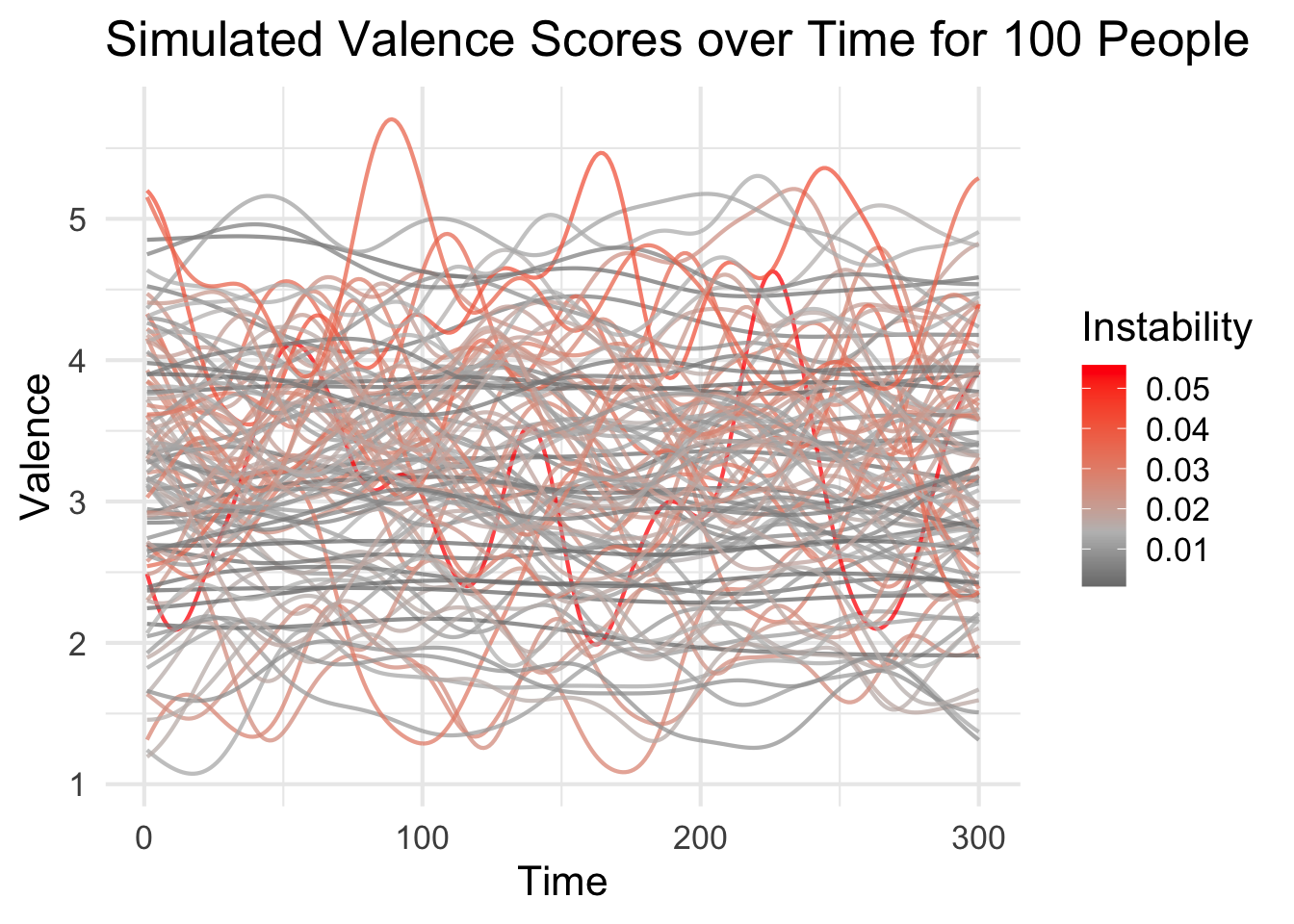
emotions_long %>%
  ggplot(aes(x = time, y = arousal, group = person, color = rmssd_a)) +
  geom_line(size = .75, alpha = .75) +
  scale_color_gradient2(low = "black", mid = "grey", high = "red", midpoint = median(emotions_long$rmssd_a)) +
  labs(x = "Time",
       y = "Arousal",
       color = "Instability",
       title = "Simulated Arousal Scores over Time for 100 People") +
  theme_minimal(base_size = 16)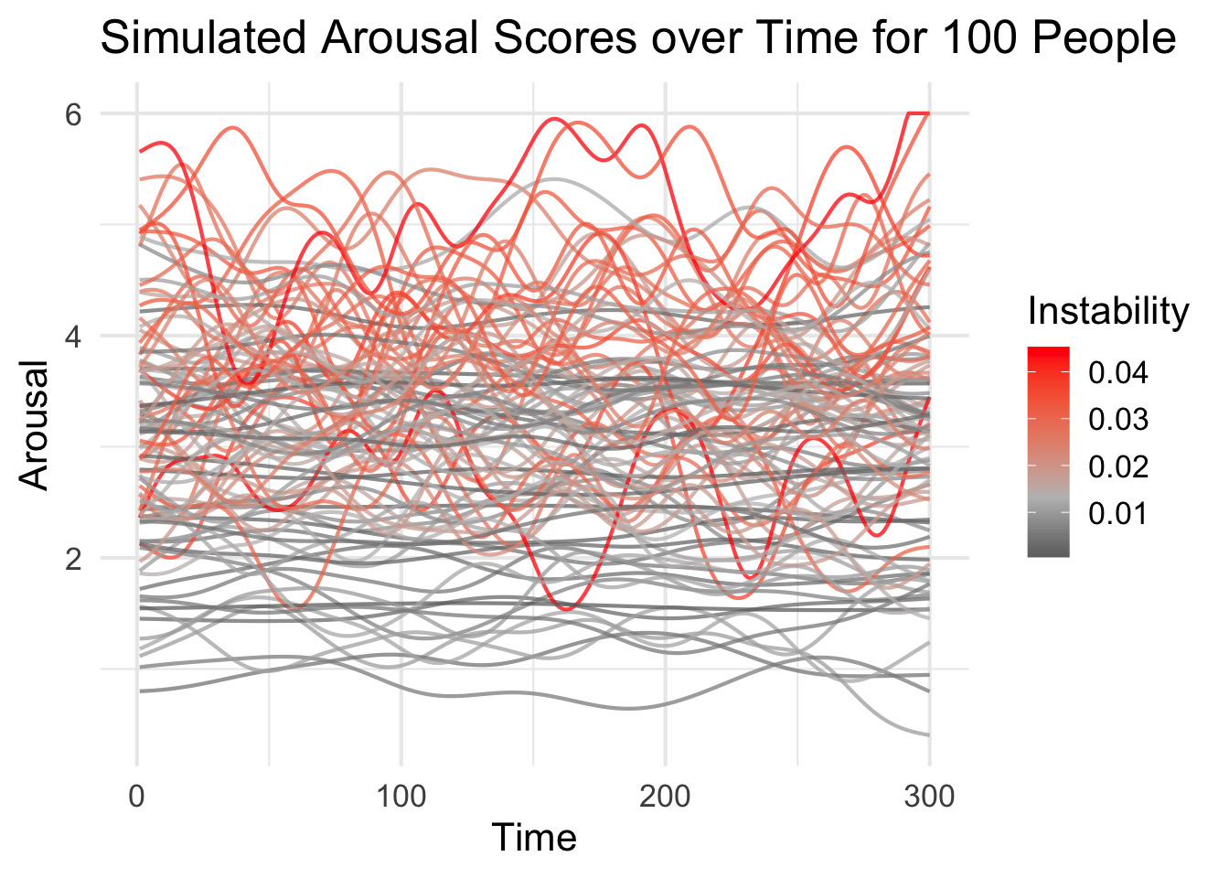
We see that some lines are fairly flat and others fluctuate more widely. More importantly, most people are somewhere in the middle.
We can get a sense of one simulated person’s affective state space as well. The goal here is to mimic the kinds of models shown in Kuppens, Oravecz, and Tuerlinckx (2010):
emotions_long %>%
  filter(person %in% sample(1:100, 6, replace = FALSE)) %>%
  ggplot(aes(x = valence, y = arousal, group = person)) +
  geom_path(size = .75) +
  scale_x_continuous(limits = c(0, 6)) +
  scale_y_continuous(limits = c(0, 6)) +
  labs(x = "Valence",
       y = "Arousal",
       title = "Affective State Space for Six Randomly Simulated People") +
  facet_wrap(~person) +
  theme_minimal(base_size = 18) +
  theme(plot.title = element_text(size = 18, hjust = .5))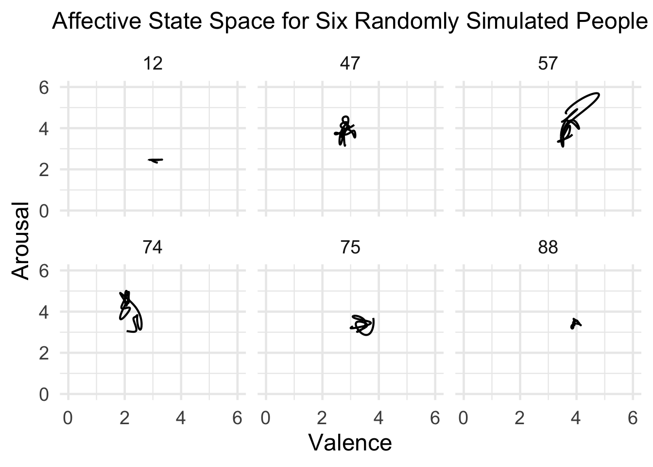
Animating the Affective State Space
To really appreciate what’s going on, we need to animate this over time. I’ll add some labels to the affective state space so that it’s easier to interpret what one might be feeling at that time. I’ll also add color to show which individuals are more unstable according to RMSSD.
library(gganimate)

p <- emotions_long %>%
  ggplot(aes(x = valence, y = arousal, color = rmssd_total)) +
  annotate("text", x = c(1.5, 4.5, 1.5, 4.5), y = c(1.5, 1.5, 4.5, 4.5), label = c("Gloomy", "Calm", "Anxious", "Happy"),
           size = 10, alpha = .50) +
  annotate("rect", xmin = 0, xmax = 3, ymin = 0, ymax = 3, alpha = 0.25, color = "black", fill = "white") +
  annotate("rect", xmin = 3, xmax = 6, ymin = 0, ymax = 3, alpha = 0.25, color = "black", fill = "white") +
  annotate("rect", xmin = 0, xmax = 3, ymin = 3, ymax = 6, alpha = 0.25, color = "black", fill = "white") +
  annotate("rect", xmin = 3, xmax = 6, ymin = 3, ymax = 6, alpha = 0.25, color = "black", fill = "white") +
  geom_point(size = 3.5) +
  scale_color_gradient2(low = "black", mid = "grey", high = "red", midpoint = median(emotions_long$rmssd_total)) +
  scale_x_continuous(limits = c(0, 6)) +
  scale_y_continuous(limits = c(0, 6)) +
  labs(x = "Valence",
       y = "Arousal",
       color = "Instability",
       title = 'Time: {round(frame_time)}') +
  transition_time(time) +
  theme_minimal(base_size = 18)

ani_p <- animate(p, nframes = 320, end_pause = 20, fps = 10, width = 550, height = 500)

ani_p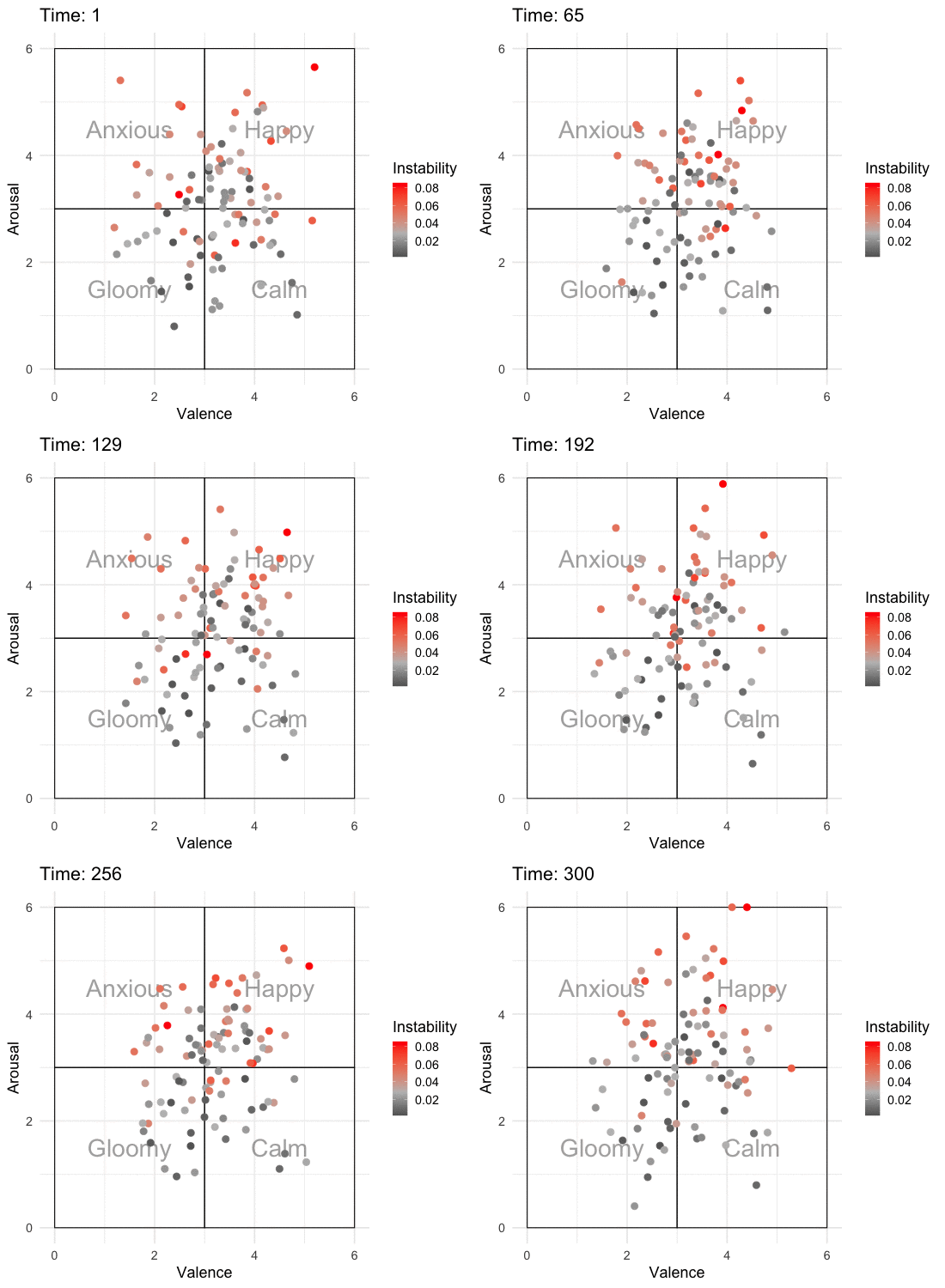
There’s a Storm Coming…
Our simulation does a pretty good job at emulating the natural ebb and flow of emotions, but we know that emotions can be far more volatile. Let’s subject our simulation to a negative event. Perhaps all 100 simulatons co-authored a paper that just got rejected. In the function simulate_affect, there’s an optional argument negative_event_time that causes a negative event to occur at the specified time. For this, we need to consider one more emotion dynamics parameter:
- Recovery rate: How quickly one recovers from an emotional event. If something bad happens, how long does it take to return to the attractor. You can see how I’ve modelled this parameter in the function above.
So we’ll run the simulation with a negative event arising at t = 150. The negative event will cause a downward spike in valence and an upward spike in arousal.
emotions_event <- simulate_affect(n = 100, time = 300, negative_event_time = 150)

emotions_event_long <- emotions_event %>%
  gather(key, value, -time) %>%
  separate(key, into = c("dimension", "person"), sep = "_") %>%
  spread(dimension, value) %>%
  group_by(person) %>%
  mutate(rmssd_v = rmssd(valence),
         rmssd_a = rmssd(arousal),
         rmssd_total = mean(rmssd_v + rmssd_a)) %>%
  ungroup()

emotions_event_long %>%
  ggplot(aes(x = time, y = valence, group = person, color = rmssd_v)) +
  geom_line(size = .75, alpha = .75) +
  scale_color_gradient2(low = "black", mid = "grey", high = "red", midpoint = median(emotions_event_long$rmssd_v)) +
  labs(x = "Time",
       y = "Valence",
       color = "Instability",
       title = "Simulated Valence Scores over Time for 100 People") +
  theme_minimal(base_size = 16)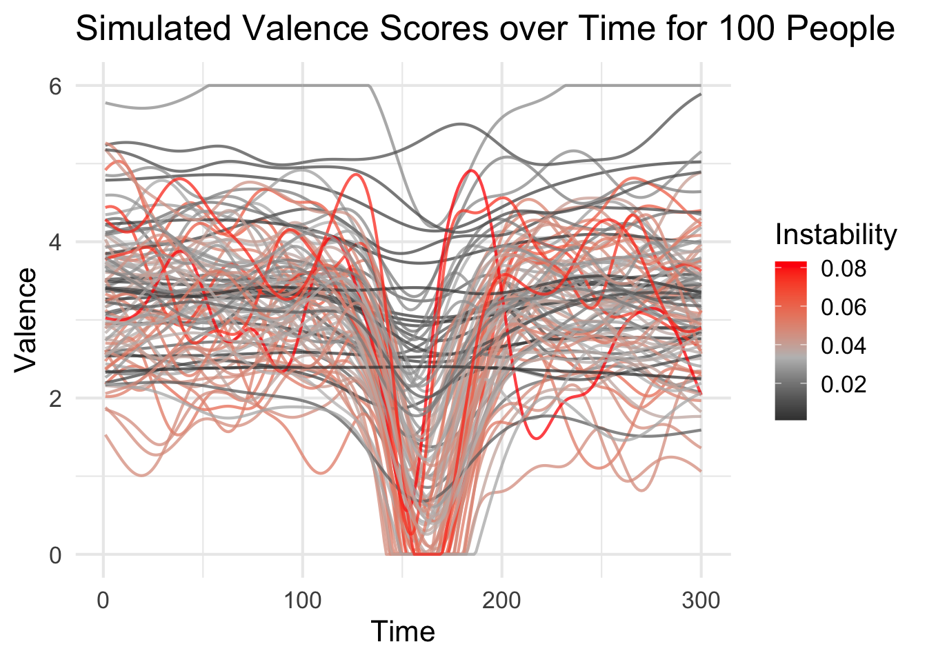
emotions_event_long %>%
  ggplot(aes(x = time, y = arousal, group = person, color = rmssd_a)) +
  geom_line(size = .75, alpha = .75) +
  scale_color_gradient2(low = "black", mid = "grey", high = "red", midpoint = median(emotions_event_long$rmssd_a)) +
  labs(x = "Time",
       y = "Arousal",
       color = "Instability",
       title = "Simulated Arousal Scores over Time for 100 People") +
  theme_minimal(base_size = 16)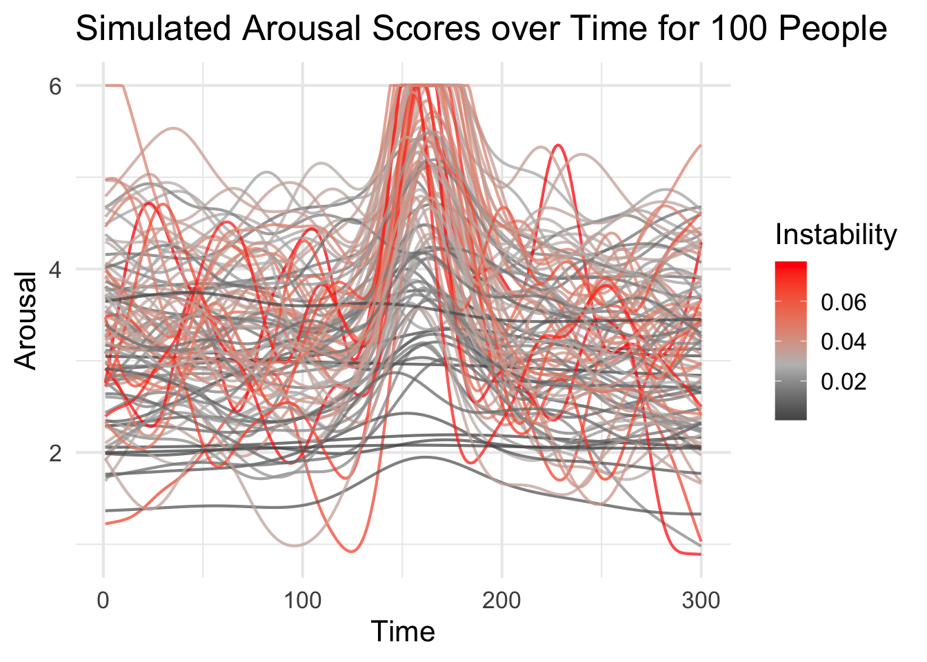
It’s pretty clear that something bad happened. Of course, some of our simulatons are unflappable, but most experienced a drop in valence and spike in arousal that we might identify as anxiety. Again, let’s visualize this evolving over time. Pay close attention to when the timer hits 150.
p2 <- emotions_event_long %>%
  ggplot(aes(x = valence, y = arousal, color = rmssd_total)) +
  annotate("text", x = c(1.5, 4.5, 1.5, 4.5), y = c(1.5, 1.5, 4.5, 4.5), label = c("Gloomy", "Calm", "Anxious", "Happy"),
           size = 10, alpha = .50) +
  annotate("rect", xmin = 0, xmax = 3, ymin = 0, ymax = 3, alpha = 0.25, color = "black", fill = "white") +
  annotate("rect", xmin = 3, xmax = 6, ymin = 0, ymax = 3, alpha = 0.25, color = "black", fill = "white") +
  annotate("rect", xmin = 0, xmax = 3, ymin = 3, ymax = 6, alpha = 0.25, color = "black", fill = "white") +
  annotate("rect", xmin = 3, xmax = 6, ymin = 3, ymax = 6, alpha = 0.25, color = "black", fill = "white") +
  geom_point(size = 3.5) +
  scale_color_gradient2(low = "black", mid = "grey", high = "red", midpoint = median(emotions_event_long$rmssd_total)) +
  scale_x_continuous(limits = c(0, 6)) +
  scale_y_continuous(limits = c(0, 6)) +
  labs(x = "Valence",
       y = "Arousal",
       color = "Instability",
       title = 'Time: {round(frame_time)}') +
  transition_time(time) +
  theme_minimal(base_size = 18)

ani_p2 <- animate(p2, nframes = 320, end_pause = 20, fps = 10, width = 550, height = 500)

ani_p2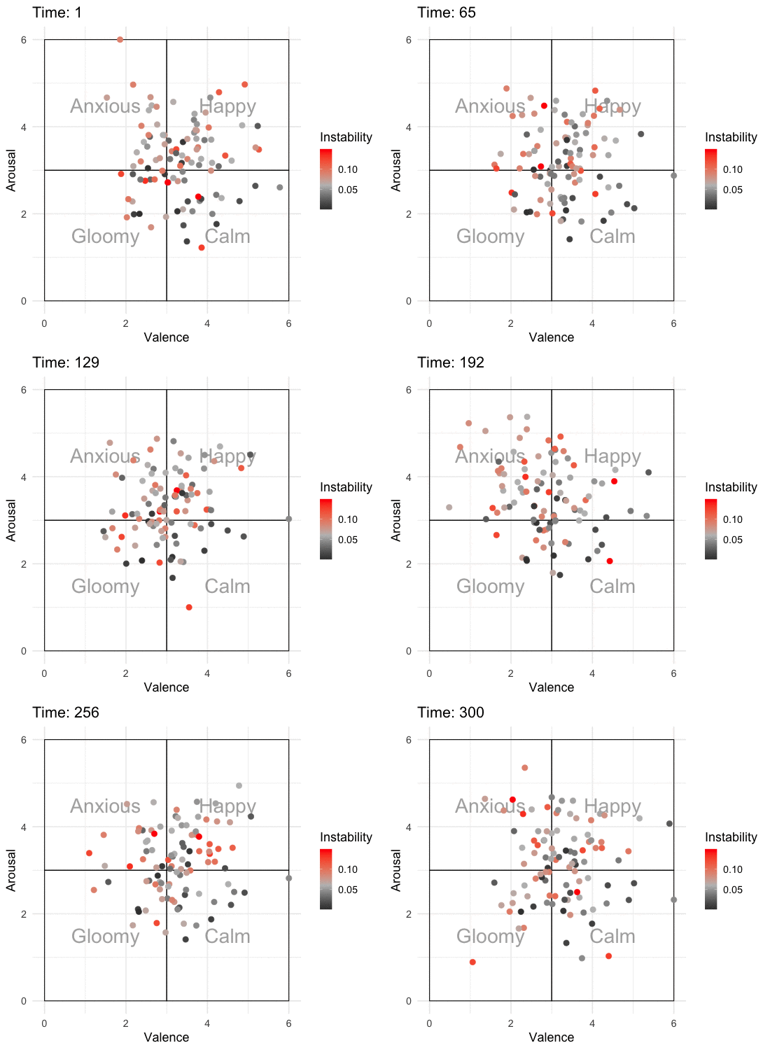
The overall picture is that some are more emotionally resilient than others. As of now, all the simulatons return to their baseline attractor, but we would realistically expect some to stay stressed or gloomy following bad news. In the coming months I’ll be looking into how to incorporate emotion regulation into the simulation. For example, maybe some of the simulatons use better coping strategies than others? I’m also interested in incorporating appraisal mechanisms that allow for different reactions depending on the type of emotional stimulus.