Visualizing a Markov Chain
A Markov Chain describes a sequence of states where the probability of transitioning from states depends only the current state. Markov chains are useful in a variety of computer science, mathematics, and probability contexts, also featuring prominently in Bayesian computation as Markov Chain Monte Carlo. Here, we’re going to look at a relatively simple breed of Markov chain and build up some intuition using simulations and animations (two of my favorite things).
The R code for simulating the Markov Chain and creating the visualizations is at the bottom of the post.
Example
Imagine a school yard with 100 children. During recess, children can either be on the soccer field or the playground. So there are two possible states for a child to be in at any given time: (1) soccer field or (2) playground. At the beginning of recess, approximately half of the children will start on the soccer field and the other half will start on the playground. But as time goes on some children will switch from the soccer field to the playground and vice versa. Let’s say we know from previous experience that at any given moment, if a child is on the soccer field they have a .10 probability (10%) of going to the playground. In contrast, if a child is on the playground they have a .05 probability (5%) of going to the soccer field. Thus, the child has a .90 and .95 probability of staying in their respective state.
This can represented pictorially. The circles (nodes) represent the two states and the arrows (edges) represent the probabilities of moving to the other state.
In this fairly simple setup, we’ll see ways of exploring how this system evolves over time.
Formal Definitions
Some terminology here: We’re describing a finite state Markov chain. This means that there is a discrete (countable) set of possible states to be in. For example, a child can be on the soccer field OR the playground and we ignore in-between states. We also say that the Markov chain is memoryless, which means that the process is only dependent on the current state of the chain. Each child’s probability of being, say, on the playground depends only on where they currently are. Let’s express these statements formally:
\[\text{Pr}(X_{n+1}=x|X_n=x_n)\]
We read this as “the probability that the next state (\(n+1\)) of the random variable \(X\) is a particular value, \(x\), depends on the current state of the random variable, \(X_n=x_n\)”.
We can also express this process as a series of matrix operations. Don’t worry if matrices aren’t your cup of tea; in this example the matrices are pretty small and the math isn’t very complicated. We start by defining a transition matrix, \(T\):
\[T=\begin{bmatrix} 0.90&0.05 \\ 0.10&0.95 \\ \end{bmatrix}\]
The elements in \(T\) correspond to the probabilities we defined earlier. For example, \(T_{1,1} = .90\) is the probability of staying on the soccer field and \(T_{2,1} = .10\) is the probability of moving from the soccer field to the playground (note that these sum to 1). Column 2 of \(T\) likewise corresponds to the probabilities of moving vs. staying when the child is on the playground.
Computing the Chain
The question we want to answer is: at the end of recess, how many children will be on the soccer field vs. the playground? Let’s start by looking at just one moment - what happens after a single iteration of the process? We don’t need to specify a time interval for each iteration (but in this example we can imagine that one iteration is ten seconds or so), we just need to be clear that the transition probabilities apply at each iteration. Here’s our equation for the first iteration:
\[X_{n=1}\begin{bmatrix} 0.90&0.05 \\ 0.10&0.95 \\ \end{bmatrix}\begin{bmatrix} 0.50\\ 0.50\\ \end{bmatrix}\]
We have our transition matrix, \(T\), from before and we’re going to matrix-multiply it with a vector containing the proportion of children present in each state (remember we said that at the beginning of recess half of the children would be on the soccer field and half on the playground). Multiplying this out we get:
\[X_{n=1}\begin{bmatrix} 0.90&0.05 \\ 0.10&0.95 \\ \end{bmatrix}\begin{bmatrix} 0.50\\ 0.50\\ \end{bmatrix} = \begin{bmatrix} 0.90\cdot0.50+0.05\cdot0.50 \\ 0.10\cdot0.50+0.95\cdot0.50 \\ \end{bmatrix} =\begin{bmatrix} 0.475\\ 0.525\\ \end{bmatrix}\]
So after one iteration we expect roughly 48 children (rounding up from \(.475\cdot100\)) to be on the soccer field and 52 children to be on the playground. If we want to see how the process unfolds over another iteration, we simply plug in the previous result and do the operation again:
\[X_{n=2}\begin{bmatrix} 0.90&0.05 \\ 0.10&0.95 \\ \end{bmatrix}\begin{bmatrix} 0.475\\ 0.525\\ \end{bmatrix} = \begin{bmatrix} 0.90\cdot0.475+0.05\cdot0.525 \\ 0.10\cdot0.475+0.95\cdot0.525 \\ \end{bmatrix} =\begin{bmatrix} 0.45\\ 0.55\\ \end{bmatrix}\]
Running the Simulation
So, analytically, this is our expected result over a couple of iterations. But we want to know how the Markov process unfolds over many iterations. We could continue doing this analytically using linear algebra, but instead we’re going to use Markov Chain Monte Carlo to obtain an empirical estimate. Markov Chain Monte Carlo is nothing more than simulating a Markov chain, like we did above but for many more iterations.
Running the chain for 100 iterations, here’s our result:
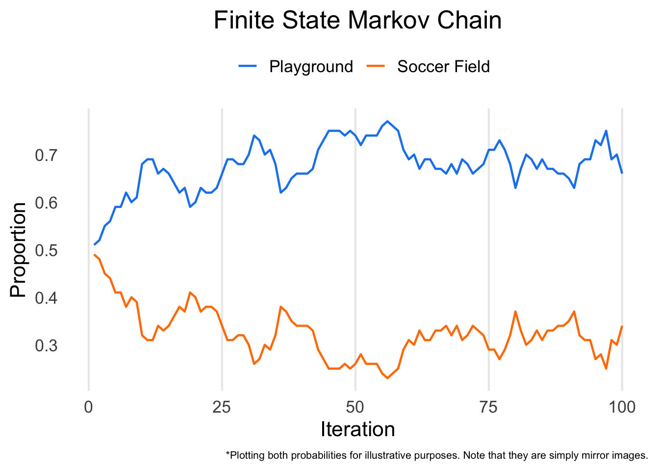
After 100 iterations of the chain, about two thirds of the children end up on the playground and one third end up on the soccer field. Note how at the beginning of the chain around the first several iterations there’s a bigger change in the proportions but then as the chain progresses it stabilizes. We would say that the chain has converged, which means that running it for more iterations probably won’t change our conclusions.
It’s worth noting that a small difference in the transition probabilities (0.05) translates into a wide difference in proportion after the chain has converged. It’s a pattern similar to phenomena described by Chaos Theory, where minor differences in starting conditions can have dramatic downstream effects.
To see this process play out in real time, here’s an animated simulation. Each dot is a child and the color corresponds to their starting location. The cluster on the left is the soccer field and the cluster on the right is the playground. I’ve also given the points a bit of random movement to simulate kids running around haphazardly on the school yard.
Adding a Third State
We aren’t just limited to two states. In fact, we can include any number of states. Let’s reimagine our example still with the soccer field and playground, but now with a third option: indoors. The transition matrix will now have dimension 3 x 3. Let’s give it the following properties:
\[T=\begin{bmatrix} 0.91&0.11&0.16 \\ 0.04&0.79&0.10 \\ 0.05&0.10&0.74 \end{bmatrix}\]
Like before, on the diagonals we have the probabilities of staying in each state. We’ll assign column 1 to be the probabilities for the soccer field, column 2 will be for the playground, and column 3 will be for indoors. We also need to assign starting probabilities. We’ll make them all roughly equal again, 0.33, 0.34, and 0.33, respectively. If we wanted to compute the estimated proportion of children in each state from one iteration to the next, we multiply \(T\) by our chosen starting probabilities:
\[\begin{bmatrix} 0.91&0.11&0.16 \\ 0.04&0.79&0.10 \\ 0.05&0.10&0.74 \end{bmatrix}\begin{bmatrix} 0.33\\ 0.34\\ 0.33 \end{bmatrix}\]
We won’t manually compute these this time… Instead, let’s run the simulation for 100 iterations.
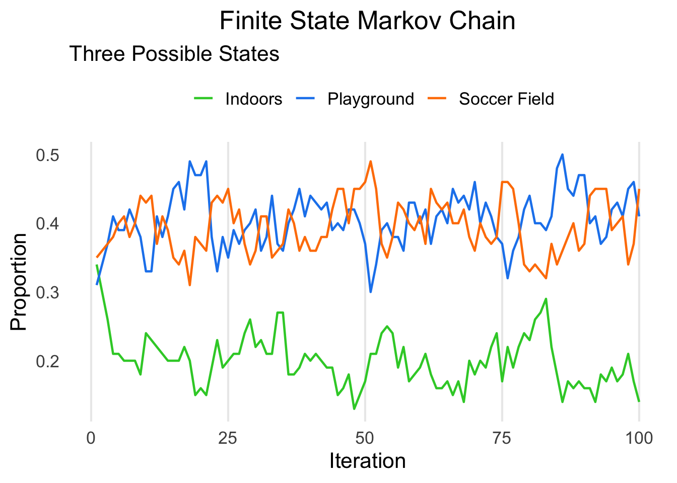
We can see that, because we made the staying probabilities for indoors relatively low, it converged to a much lower value compared to its starting value.
Here’s an animated version of the simulation slightly more sped up:
What about Zero Probability Transitions?
We can do some pretty interesting things when we constrain some transition probabilities to be zero. For a moment, let’s imagine in our example that all children start indoors when recess begins and to get to the soccer field they need to go through the playground. In other words, it is impossible to go from indoors directly to the soccer field and vice versa.
Our transition matrix might look something like this:
\[T=\begin{bmatrix} 0.85&0.13&0 \\ 0.15&0.85&0.05 \\ 0&0.02&0.95 \end{bmatrix}\begin{bmatrix} 1\\ 0\\ 0 \end{bmatrix}\]
Now because all children start indoors the points are all green.
So there’s a brief look at how Markov chains work. Markov chains have vast applications, but where I come across them most often is their role in Bayesian computations. We didn’t go into this application here, but hopefully after this you have an intuitive grasp of what a Markov chain is.
Continue reading if you want to see how I coded the Markov chain and the animations!
Behind the Scenes
Below is the annotated code for creating and animating the Markov chain. Feel free to customize it to your heart’s content.
Building the Simulation
Here’s the function I created to run the Markov-based simulation. In our example, n is the number of children in the simulation. We specify the number of iterations and provide starting probabilities for each of the states and transition probabilities for the probability of moving from a state to another state. Note that in the binary case we don’t actually have to supply a matrix since we can leverage inverse probability.
Binary State
library(tidyverse) # includes ggplot2, dplyr, and others
library(plotly)
markov1 <- function(n = 100, iter = 100, start_probs = c(.50, .50), trans_probs = c(.10, .05), plot_prob = TRUE) {
#Check to see if probability entries are valid.
if(sum(start_probs) != 1 | any(start_probs < 0))
stop("start_probs must be non-negative and sum to 1.")
if(sum(trans_probs) > 1 | any(trans_probs < 0))
stop("trans_probs must be non-negative and not sum to greater than 1.")
dt <- matrix(NA, nrow = iter, ncol = n) # Initialize matrix to hold iterations
# Run chain
for(i in 1:iter) {
for(j in 1:n) {
if(i == 1) { # if we're at the beginning of the simulation
dt[i, j] <- sample(x = c(0, 1), size = 1, prob = start_probs)
} else {
if(dt[i - 1, j] == 0) { # if the previous state was 0
dt[i, j] <- sample(x = c(0, 1), size = 1, prob = c(1 - trans_probs[1], trans_probs[1]))
} else { # if the previous state was not 0, we know it must have been 1
dt[i, j] <- sample(x = c(1, 0), size = 1, prob = c(1 - trans_probs[2], trans_probs[2]))
}
}
}
}
# Plot results?
if(plot_prob) {
df <- data.frame(x = 1:iter, y = apply(dt, 1, mean))
p <- ggplot(df, aes(x, y)) +
geom_line() +
labs(x = "Iteration",
y = "Prop.") +
theme_minimal(base_size = 16)
show(p)
}
# Return chain as dataframe
return(as.data.frame(dt))
}
df <- markov1() # execute the functionAnimating the Binary State Markov Chain
I used Plotly to generate the animations. In the past I’ve tended toward gganimate because it integrates really well with ggplot, but I find the result from Plotly to be sleeker.
I’ve added a few aesthetic elements. First, some jittering to the points to make them more visible. Second, I added some lag dependency (using dplyr’s lag function) and smoothing using the base spline function. This actually adds extra values to create the smooth transition, so we need to be careful with it.
The plotly code itself is fairly straightforward. A good resource for learning plotly in R is through their website.
df_long <- df %>%
rowid_to_column(var = "iter") %>%
pivot_longer(cols = V1:V100) %>%
group_by(name) %>%
mutate(x_jitter = rnorm(n(), 0, .025),
x_jitter = x_jitter + lag(x_jitter, default = 0),
x = value + x_jitter,
y = rnorm(1, 0, .01),
y = lag(y, default = 0) + rnorm(n(), 0, .01)) %>%
group_map(~ {
value = .$value
name = .y
x = spline(.$iter, .$x)$y
y = spline(.$iter, .$y)$y
data.frame(name, value, x, y)
})
df_full <- do.call(rbind, df_long) %>%
group_by(name) %>%
mutate(initial = value[1],
iter = row_number()) %>%
group_by(iter) %>%
mutate(prop1 = mean(value),
prop0 = 1 - prop1)
anim1 <- df_full %>%
plot_ly(
x = ~x,
y = ~y,
color = ~factor(initial),
size = 2,
colors = c("#FF7F00", "#1C86EE"),
frame = ~iter,
type = 'scatter',
mode = 'markers',
showlegend = FALSE
)
anim1 <- anim1 %>%
add_text(x = 1, y = .025, text = ~prop1, textfont = list(color = "#1C86EE", opacity = .6)) %>%
add_text(x = 0, y = .025, text = ~prop0, textfont = list(color = "#FF7F00", opacity = .6))
ax <- list(
zeroline = FALSE,
showline = FALSE,
showticklabels = FALSE,
showgrid = FALSE,
title = ""
)
anim1 <- anim1 %>%
layout(xaxis = ax, yaxis = ax) %>%
animation_opts(redraw = FALSE) %>%
animation_slider(hide = TRUE) %>%
animation_button(x = .6, y = .10, showactive = TRUE, label = "Run Simulation") %>%
config(displayModeBar = FALSE, scrollZoom = FALSE, showTips = FALSE)
anim1Building the Triple State Simulation
The function for three states builds on the original binary state function. All that really needs to change is that the transition probabilities are captured in a matrix (although as we saw above, the binary state is technically a matrix too but we just don’t need to express it that way).
set.seed(200322)
markov2 <- function(n = 100, iter = 100, start_probs = c(.33, .33, .34), trans_probs = matrix(c(.91, .11, .16,
.04, .79, .10,
.05, .10, .74), ncol = 3),
plot_prob = TRUE) { # Here we have a full non-zero transition matrix.
#Check to see if probability entries are valid.
if(sum(start_probs) != 1 | any(start_probs < 0))
stop("start_probs must be non-negative and sum to 1.")
if(any(apply(trans_probs, 1, sum) != 1))
stop("trans_probs matrix rows must sum to 1.")
if(any(trans_probs < 0))
stop("elements of trans_probs must be non-negative")
dt <- matrix(NA, nrow = iter, ncol = n) # Initialize matrix to hold iterations
# Run chain
for(i in 1:iter) {
for(j in 1:n) {
if(i == 1) { # if we're at the beginning of the simulation
dt[i, j] <- sample(x = c(0, 1, 2), size = 1, prob = start_probs)
} else {
if(dt[i - 1, j] == 0) { # if the previous state was 0
dt[i, j] <- sample(x = c(0, 1, 2), size = 1, prob = trans_probs[,1])
} else if (dt[i - 1, j] == 1) { # if the previous state was 1
dt[i, j] <- sample(x = c(0, 1, 2), size = 1, prob = trans_probs[,2])
} else {
dt[i, j] <- sample(x = c(0, 1, 2), size = 1, prob = trans_probs[,3])
}
}
}
}
# Plot results?
if(plot_prob) {
df <- data.frame(x = 1:iter,
n0 = apply(subset(dt == 0), 1, sum),
n1 = apply(subset(dt == 1), 1, sum),
n2 = apply(subset(dt == 2), 1, sum))
p <- df %>%
pivot_longer(cols = c(n0, n1, n2)) %>%
ggplot(aes(x, value, color = name)) +
geom_line() +
scale_color_discrete(labels = c("0", "1", "2")) +
labs(x = "Iteration",
y = "Prop.") +
theme_minimal(base_size = 16)
show(p)
}
# Return chain as dataframe
return(as.data.frame(dt))
}
df2 <- markov2()Animating the Triple State Markov Chain
Animation proceeds much as before. I decided against the smoothing this time around because it started to look a bit too messy with three states.
df_long2 <- df2 %>%
rowid_to_column(var = "iter") %>%
pivot_longer(cols = V1:V100) %>%
group_by(name) %>%
mutate(x = value + rnorm(1, 0, .10) + rnorm(n(), 0, .01),
y = value %% 2 + rnorm(1, 0, .10) + rnorm(n(), 0, .01),
initial = value[1],
is_0 = ifelse(value == 0, TRUE, FALSE),
is_1 = ifelse(value == 1, TRUE, FALSE)) %>%
group_by(iter) %>%
mutate(prop0 = mean(is_0),
prop1 = mean(is_1),
prop2 = 1 - prop0 - prop1) %>%
ungroup()
anim2 <- df_long2 %>%
plot_ly(
x = ~x,
y = ~y,
color = ~factor(initial),
size = 2,
colors = c("#32CD32", "#1C86EE", "#FF7F00"),
frame = ~iter,
type = 'scatter',
mode = 'markers',
showlegend = FALSE
)
anim2 <- anim2 %>%
add_text(x = 0, y = .35, text = ~prop0, textfont = list(color = "#32CD32", size = 24, opacity = .6)) %>%
add_text(x = 1, y = 1.25, text = ~prop1, textfont = list(color = "#1C86EE", size = 24, opacity = .6)) %>%
add_text(x = 2, y = .35, text = ~prop2, textfont = list(color = "#FF7F00", size = 24, opacity = .6))
ax2 <- list(
zeroline = FALSE,
showline = FALSE,
showticklabels = FALSE,
showgrid = FALSE,
title = ""
)
anim2 <- anim2 %>%
layout(xaxis = ax2, yaxis = ax2) %>%
animation_opts(redraw = FALSE) %>%
animation_slider(hide = TRUE) %>%
animation_button(x = .6, y = .10, showactive = TRUE, label = "Run Simulation") %>%
config(displayModeBar = FALSE, scrollZoom = FALSE, showTips = FALSE)
anim2Here’s the zero probability version:
df3 <- markov2(iter = 100, start_probs = c(1, 0, 0), trans_probs = matrix(c(.85, .13, 0,
.15, .85, .05,
0, .02, .95), ncol = 3),
plot_prob = FALSE)
df_long3 <- df3 %>%
rowid_to_column(var = "iter") %>%
pivot_longer(cols = V1:V100) %>%
group_by(name) %>%
mutate(x = value + rnorm(1, 0, .05) + rnorm(n(), 0, .01),
y = rnorm(1, 0, .025) + rnorm(n(), 0, .01),
initial = value[1],
is_0 = ifelse(value == 0, TRUE, FALSE),
is_1 = ifelse(value == 1, TRUE, FALSE)) %>%
group_by(iter) %>%
mutate(prop0 = round(mean(is_0), 2),
prop1 = round(mean(is_1), 2),
prop2 = round(1 - prop0 - prop1, 2)) %>%
ungroup()
anim3 <- df_long3 %>%
plot_ly(
x = ~x,
y = ~y,
size = 2,
color = ~factor(initial),
colors = c("#32CD32", "#32CD32", "#32CD32"),
frame = ~iter,
type = 'scatter',
mode = 'markers',
showlegend = FALSE
)
anim3 <- anim3 %>%
add_text(x = 0, y = .15, text = ~prop0, textfont = list(color = "#32CD32", size = 32, opacity = .6)) %>%
add_text(x = 1, y = .15, text = ~prop1, textfont = list(color = "#1C86EE", size = 32, opacity = .6)) %>%
add_text(x = 2, y = .15, text = ~prop2, textfont = list(color = "#FF7F00", size = 32, opacity = .6))
ax3 <- list(
zeroline = FALSE,
showline = FALSE,
showticklabels = FALSE,
showgrid = FALSE,
title = ""
)
anim3 <- anim3 %>%
layout(xaxis = ax3, yaxis = ax3) %>%
animation_opts(redraw = FALSE) %>%
animation_slider(hide = TRUE) %>%
animation_button(x = .6, y = .10, showactive = TRUE, label = "Run Simulation") %>%
config(displayModeBar = FALSE, scrollZoom = FALSE, showTips = FALSE)
anim3Spot any errors? Have any suggestions? Send me a quick email (contact info below).