Bayesian Varying Effects Models in R and Stan
In psychology, we increasingly encounter data that is nested. It is to the point now where any quantitative psychologist worth their salt must know how to analyze multilevel data. A common approach to multilevel modeling is the varying effects approach, where the relation between a predictor and an outcome variable is modeled both within clusters of data (e.g., observations within people, or children within schools) and across the sample as a whole. And there is no better way to analyze this kind of data than with Bayesian statistics. Not only does Bayesian statistics give solutions that are directly interpretable in the language of probability, but Bayesian models can be infinitely more complex than Frequentist ones. This is crucial when dealing with multilevel models, which get complex quickly.
A preview of what’s to come:
Stan is the lingua franca for programming Bayesian models. You code your model using the Stan language and then run the model using a data science language like R or Python. Stan is extremely powerful, but it is also intimidating even for an experienced programmer. In this post, I’ll demonstrate how to code, run, and evaluate multilevel models in Stan.
I assume a basic grasp of Bayesian logic (i.e., you understand priors, likelihoods, and posteriors). I’ve written some content introducing these terms here if you want to check that out first. I also assume familiarity with R and the tidyverse packages (in particular, ggplot2, dplyr, and purrr).
You’ll need to install the rstan package to follow along. This installation is more involved than typical R packages. The instructions on Stan’s website will help you get started.
One more note before we dive in. If you’re just starting out with Bayesian statistics in R and you have some familiarity with running Frequentist models using packages like lme4, nlme, or the base lm function, you may prefer starting out with more user-friendly packages that use Stan as a backend, but hide a lot of the complicated details. Some time back I wrote up a demonstration using the brms package, which allows you to run Bayesian mixed models (and more) using familiar model syntax. I started with brms and am gradually building up competency in Stan. Stan is the way to go if you want more control and a deeper understanding of your models, but maybe brms is a better place to start. Regardless, I’ll try to give intuitive explanations behind the Stan code so that you can hopefully start writing it yourself someday. Don’t be discouraged if it doesn’t sink in right away.
Simulating the Data
We are creating repeated measures data where we have several days of observations for a group of participants (each denoted by pid). Our outcome variable is y and our continuous predictor is x. We’ll imagine that the days of observation are random so we won’t need to model it as a grouping variable.
Here’s the code to simulate the data we’ll use in this post. For now, it’s just enough to copy the code and run it so that you’ll have the data. This code will make more sense once we start working with the models.
library(tidyverse) # for ggplot2, dplyr, purrr, etc.
theme_set(theme_bw(base_size = 14)) # setting ggplot2 theme

library(mvtnorm)

set.seed(12407) # for reproducibility

# unstandardized means and sds
real_mean_y <- 4.25
real_mean_x <- 3.25
real_sd_y <- 0.45
real_sd_x <- 0.54

N <- 30 # number of people
n_days <- 7 # number of days
total_obs <- N * n_days

sigma <- 1 # population sd
beta <- c(0, 0.15) # average intercept and slope
sigma_p <- c(1, 1) # intercept and slope sds
rho <- -0.36 # covariance between intercepts and slopes

cov_mat <- matrix(c(sigma_p[1]^2, sigma_p[1] * sigma_p[2] * rho, sigma_p[1] * sigma_p[2] * rho, sigma_p[2]^2), nrow = 2)
beta_p <- rmvnorm(N, mean = beta, sigma = cov_mat) # participant intercepts and slopes

x <- matrix(c(rep(1, N * n_days), rnorm(N * n_days, 0, 1)), ncol = 2) # model matrix
pid <- rep(1:N, each = n_days) # participant id

sim_dat <- map_dfr(.x = 1:(N * n_days), ~data.frame(
  mu = x[.x, 1] * beta_p[pid[.x], 1] + x[.x, 2] * beta_p[pid[.x], 2],
  pid = pid[.x],
  x = x[.x, 2]
))

sim_dat$y <- rnorm(210, sim_dat$mu, sigma) # creating observed y from mu and sigma

dat <- sim_dat %>%
  select(-mu) %>% # removing mu
  mutate(y = real_mean_y + (y * real_sd_y), # unstandardize
         x = real_mean_x + (x * real_sd_x)) # unstandardize
We now have a data frame that is very much like something you would come across in psychology research. Let’s perform a quick check on the data to see that the simulation did what we wanted it to.
dat %>%
  ggplot(aes(x = x, y = y, group = pid)) +
  geom_point(color = "cadetblue4", alpha = 0.80) +
  geom_smooth(method = 'lm', se = FALSE, color = "black") +
  facet_wrap(~pid)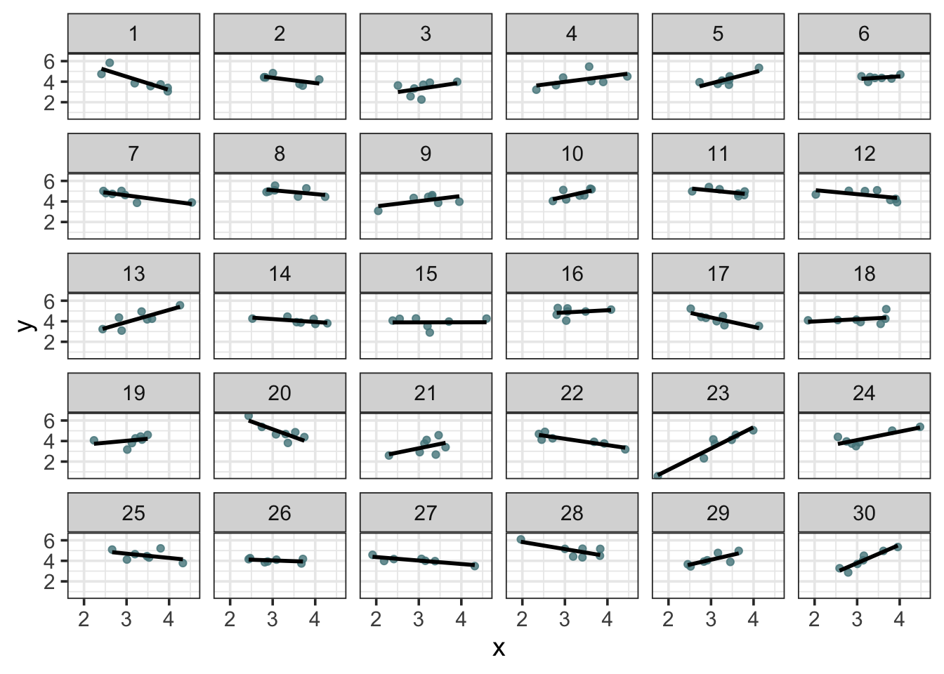
We can see a good amount of clustering at the participant level. Ok, so we have our data, now let’s analyze it.
Bayesian Workflow
A good Bayesian analysis includes the following steps:
- Prior predictive checks.
- Model execution using Markov Chain Monte Carlo.
- Posterior predictive checks.
- Model comparison
We’ll focus in this post of the first three, saving model comparison for another day. For the models in this post, I’ll give examples of each of the three steps. Steps 1 and 3 strongly leverage plotting techniques, so we’ll make good use of ggplot2.
Example with Simple Linear Regression
It’s been said that linear regression is the ‘Hello World’ of statistics. To see the Bayesian workflow in action and get comfortable, we’ll start with a simple (albeit inappropriate) model for this data - one in which we completely ignore the grouping of the data within participants and instead treat each observation as completely independent from the others. This is not the way to analyze this data, but I use it as a simple demonstration of how to construct Stan code.
In mathematical notation, here is our simple linear regression model:
\[ \begin{aligned} y_i \sim \text{Normal}(\mu, \sigma) \\ \mu_i= \beta_0 + \beta_1 x_i \\ \beta_0 \sim \text{Normal}(0, 1) \\ \beta_1 \sim \text{Normal}(0, 1) \\ \sigma \sim \text{Exponential}(1) \end{aligned} \]
I give full credit to McElreath’s brilliant Statistical Rethinking (2020) for introducing me to this way of writing out models. It’s a bit jarring at first; myself having become accustomed to model formulas as one-liners. But once you understand it it’s a really elegant way of expressing the model. We start by expressing how the outcome variable, \(y\), is distributed: it has a deterministic part, \(\mu\) (the mean), and an error, \(\sigma\) (the standard deviation). \(\mu_i\) is the expected value for each observation, and if you have encountered regressions before, you know that the expected value for a given observation is the intercept, \(\beta_0\) + \(\beta_1\) times the predictor \(x_i\).
We then assign priors to the parameters. Priors encode our knowledge and uncertainty about the data before we run the model. We don’t use priors to get a desired result, we use priors because it makes sense. Without priors, our model initially ‘thinks’ that the data is just as likely to come from a normal distribution with a mean of 0 and sigma of 1 as it is to come from a distribution with a mean of 1,000 and a sigma of 400. True, the likelihood function (i.e., the probability of the data given the model) will sort things out when we have sufficient data, but we’ll see that priors play a particularly important role when we move on to varying effects models.
The model formula above includes priors for \(\beta_0\), \(\beta_1\), and \(\sigma\). But how do we know these are reasonable priors? (True, these are conventional priors and pose little threat, but let’s assume we don’t know that.). We’re going to perform some visual checks on our priors to ensure they are sensible.
Prior Predictive Checks
First, let’s see what different prior distributions look like. We’ll use conventional normal priors on \(\beta_0\) and \(\beta_1\). We’ll try out three different normal distributions.
We create a grid of evenly spaced values. We then want to see the likelihood of these xs in the context of three normal distributions with the same mean but different standard deviations. We use the map_dfr function from the purrr package to iterate over the three different distributions and store the result in a data frame.
grid <- seq(-3, 3, length.out = 1000) # evenly spaced values from -3 to 3

b0_prior <- map_dfr(.x = c(0.5, 1, 2), ~ data.frame( # .x represents the three sigmas
  grid = grid,
  b0 = dnorm(grid, mean = 0, sd = .x)),
  .id = "sigma_id")

# create friendlier labels
b0_prior <- b0_prior %>%
  mutate(sigma_id = factor(sigma_id, labels = c("normal(0, 0.5)",
                                                "normal(0, 1)",
                                                "normal(0, 2)")))

ggplot(b0_prior, aes(x = grid, y = b0)) +
  geom_area(fill = "cadetblue4", color = "black", alpha = 0.90) +
  scale_x_continuous(expand = c(0, 0)) +
  scale_y_continuous(expand = c(0, 0), limits = c(0, 0.85)) +
  labs(x = NULL,
       y = "probability density",
       title = latex2exp::TeX("Possible $\\beta_0$ (intercept) priors")) +
  facet_wrap(~sigma_id, nrow = 3)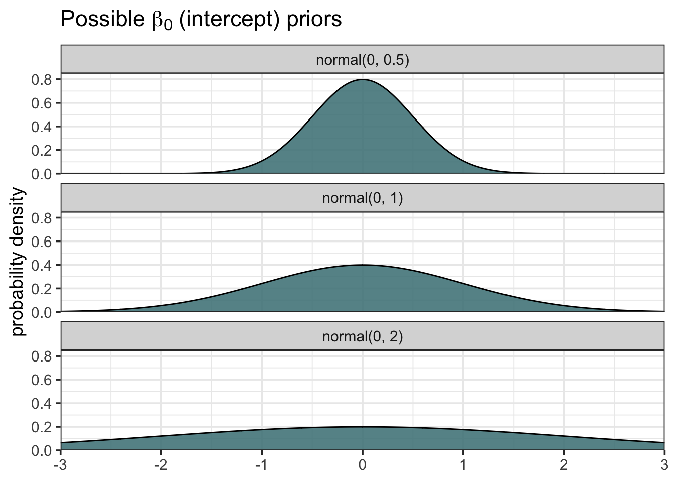
We can see that the three distributions vary in terms of how spread out they are. We might say that the top distribution with mean 0 and sd 0.5 is more “confident” about the probability of values close to zero, or that it is more skeptical about extreme values. Flatter distributions allocate probability more evenly and are therefore more open to extreme values.
This is all well and good, but looking at the raw probability densities doesn’t tell us much about what the priors assume about the data. We need to look at what kind of data is compatible with the priors. So this time we’ll generate regression lines from the \(\beta_0\) and \(\beta_1\) priors. Remember, all you need to create a line is an intercept and a slope!
The trick this time is to generate intercepts and slopes from the different normal distributions. Again, we’ll stick with three different distributions, but now we use map2_dfr to iterate over a \(\beta_0\) prior and a \(\beta_1\) prior.
b0b1 <- map2_df(.x = c(0.5, 1, 2), .y = c(0.25, 0.5, 1), ~ data.frame(
  b0 = rnorm(100, mean = 0, sd = .x),
  b1 = rnorm(100, mean = 0, sd = .y)), .id = "sigma_id"
)

# create friendlier labels
b0b1 <- b0b1 %>%
  mutate(sigma_id = factor(sigma_id, labels = c("b0 ~ normal(0, 0.5); b1 ~ normal(0, 0.25)",
                                                "b0 ~ normal(0, 1); b1 ~ normal(0, 0.50)",
                                                "b0 ~ normal(0, 2); b1 ~ normal(0, 1)")))

ggplot(b0b1) +
  geom_abline(aes(intercept = b0, slope = b1), color = "cadetblue4", alpha = 0.75) +
  scale_x_continuous(limits = c(-2, 2)) +
  scale_y_continuous(limits = c(-3, 3)) +
  labs(x = "x",
       y = "y",
       title = latex2exp::TeX("Sampling of lines from $\\beta_0$ and $\\beta_1$ priors")) +
  facet_wrap(~sigma_id, nrow = 3)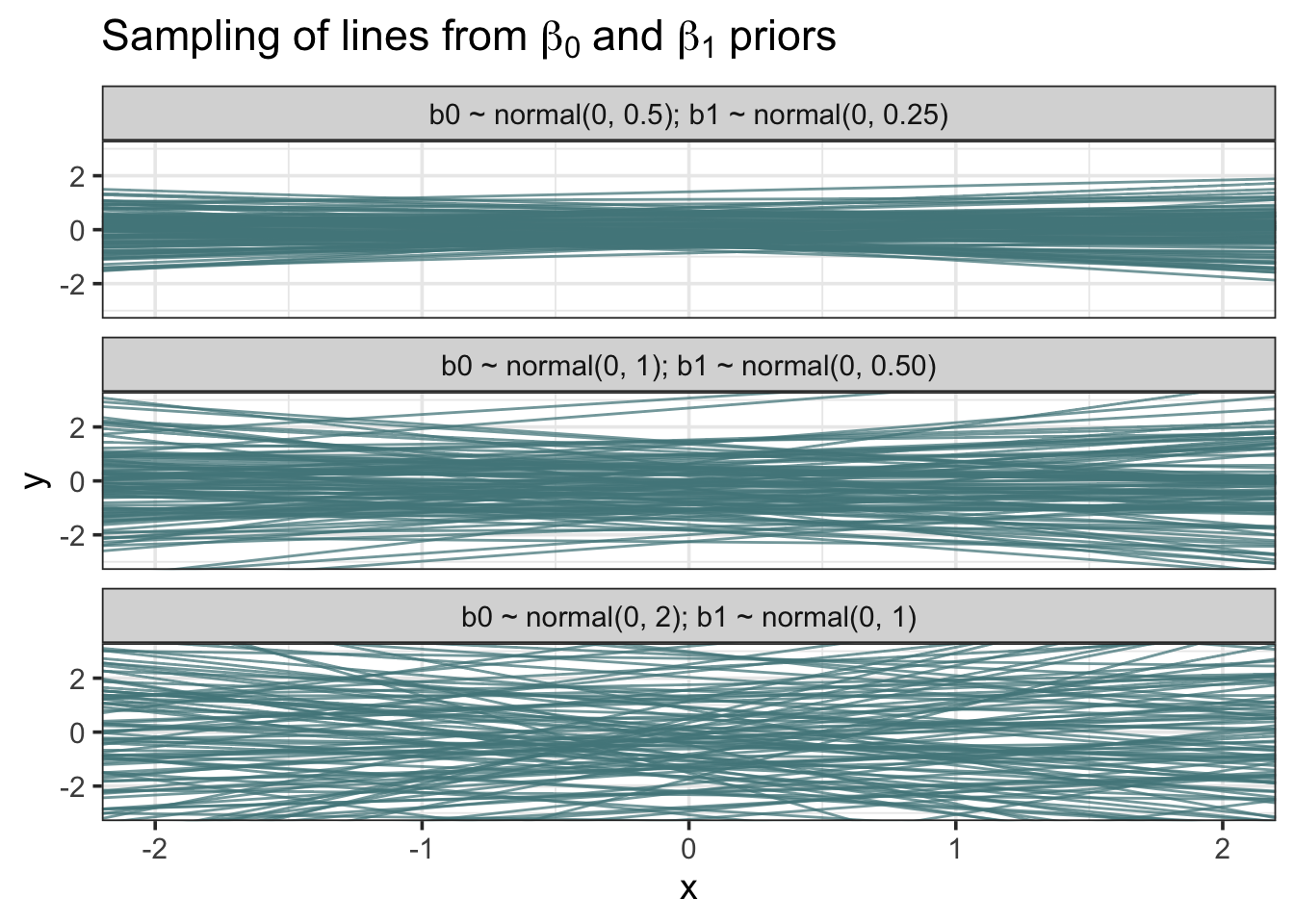
The more restrictive set of priors on the top constrains the lines to have intercepts and slopes close to zero, and you can see that the lines vary little from one another. In contrast, the weaker priors allow a much greater variety of intercept/slope combinations.
Later we’ll see how to generate actual data from the priors, but for now let’s go ahead with the priors I’ve provided in the model formula and begin coding the model in Stan!
Stan Basics
Every Stan model code must contain the following three blocks:
- Data - where you define the data and the dimensions of the data.
- Parameters - where you describe the unknown parameters that you want to estimate.
- Model - where you list the priors and define the likelihood function for the model.
For an R user, the best way to write Stan code is to use RStudio’s built-in Stan file editor. If you have Stan installed, when you select the drop down options for a new file in RStudio, you can select ‘Stan file’. This lets you take advantage of autocompletion and syntax error detection.
In the examples to follow I’ll make it clear which code snippets are in Stan code with a // STAN CODE marker at the beginning of the block (// denotes a comment and is not evaluated). For each model, I’ll explain each code block separately and then give the model code as a whole. Note that unlike in R, you cannot run Stan code lines one by one and see their output - a Stan file is only evaluated (compiled) when you execute the rstan function in R, which we’ll see later.
Data
The data block is where we define our observed variables. We also need to define lengths/dimensions of stuff, which can seem strange if you’re used to R or Python. We first declare an integer variable N to be the number of observations: int N; (note the use of semicolon to denote the end of a line). I’m also declaring an integer K, which is the number of predictors in our model. Note that I’m including the intercept in this count, so we end up with 2 predictors (2 columns in the model matrix).
Now we supply actual data. We write matrix[N, K] to tell Stan that x is a \(N \times K\) matrix. y is easier - just a vector of length \(N\).
// STAN CODE
data {
  int N; // number of observations
  int K; // number of predictors + intercept
  matrix[N, K] x; // x vector
  vector[N] y; // y vector
}
Parameters
Now we tell Stan the parameters in our model. These are the unobserved variables that we want to estimate. In this example, we have 3 parameters: \(\beta_0\), \(\beta_1\) and \(\sigma\). Like before, we first tell Stan the type of data this parameter will contain - in this case, \(\beta_0\) and \(\beta_1\) are contained in a vector of length \(K\) that we will sensibly call beta. \(\sigma\) will just be a single real value (“real” means that the number can have a decimal point). We use <lower=0> to constrain it to be positive because it is impossible to have negative standard deviation.
// STAN CODE
parameters {
  vector[K] beta; // intercept and slope parameters
  real<lower=0> sigma; // constrained to be positive
}
Model
The model block is where the action is at. We start with our priors. There should be a prior for each parameter declared above.
// STAN CODE
model {
  vector[N] mu; // declaring a mu vector

  // priors
  beta ~ normal(0, 1); // declares the same prior for intercept and slope
  sigma ~ exponential(1); // using an exponential prior on sigma

  // likelihood
  for(i in 1:N) {
    mu[i] = x[i] * beta; // * is matrix multiplication in this context, where x[i] is the first row of x
  }

  y ~ normal(mu, sigma);
}
The part above where we define \(\mu\) (mu[i]) can seem a bit strange. You may be wondering how the intercept and slope factor into this calculation. The compact notation hides some of the magic, which really isn’t very magical since it’s just a dot product. In matrix form, it looks like this:
\[\mu_i=\begin{bmatrix} 1&x_i\\ \end{bmatrix} \begin{bmatrix} \beta_0\\ \beta_1 \end{bmatrix}\]
where \(1\) is the intercept and \(x_i\) is the \(i^{th}\) value of the variable \(x\). Computing this dot product for each participant i gives you an expected value mu for each participant.
Full Stan Code
The full Stan code looks like this:
// STAN CODE
data {
  int N; // number of observations
  int K; // number of predictors + intercept
  matrix[N, K] x; // matrix of predictors
  vector[N] y; // y vector
}

parameters {
  vector[K] beta; // intercept and slope parameters
  real<lower=0> sigma; // constrained to be positive
}

model {
  vector[N] mu; // declaring a mu vector

  // priors
  beta ~ normal(0, 1); // declares the same prior for intercept and slope
  sigma ~ exponential(1); // using an exponential prior on sigma

  // likelihood
  for(i in 1:N) {
    mu[i] = x[i] * beta; // * is matrix multiplication in this context
  }

  y ~ normal(mu, sigma);
}
Saving this file will give it a .stan file extension. It’s a good idea to save it in your project directory. I’ll name this model "mod1.stan".
Running the Model
Now we go back to R to run the model. If you haven’t already, load up rstan.
library(rstan)We need to put the data in a list for Stan. Everything that we declared in the data block of our Stan code should be entered into this list. We’ll also standardize the variables, so that they match up with our priors.
stan_dat <- list(
  N = nrow(dat), # using nrow() to get the number of rows (observations)
  K = 2, # (1) intercept, (2) slope
  x = matrix(c(rep(1, nrow(dat)), scale(dat$x)), ncol = 2), # model matrix (x standardized)
  y = as.vector(scale(dat$y)) # standardized outcome. convert to vector to avoid issues with scale function
)
Finally, we use the function stan to run the model. We set chains and cores to 4, which will allow us to run 4 Markov chains in parallel.
stan_fit1 <- stan(file = "mod1.stan",
                  data = stan_dat,
                  chains = 4, cores = 4)
Evaluating the Model
We can take a look at the parameters in the console by printing the model fit. We get posterior means, standard errors, and quantiles for each parameter. We also get things called n_eff and Rhat. These are indicators of how well Stan’s engine explored the parameter space (if this is cryptic, that’s ok), It’s enough for now to know that when Rhat is 1, things are good.
stan_fit1## Inference for Stan model: mod1.
## 4 chains, each with iter=2000; warmup=1000; thin=1;
## post-warmup draws per chain=1000, total post-warmup draws=4000.
##
## mean se_mean sd 2.5% 25% 50% 75% 97.5% n_eff Rhat
## beta[1] 0.00 0.00 0.07 -0.13 -0.05 0.00 0.05 0.13 4608 1
## beta[2] 0.09 0.00 0.07 -0.05 0.04 0.09 0.14 0.22 4188 1
## sigma 1.00 0.00 0.05 0.91 0.97 1.00 1.03 1.10 3928 1
## lp__ -106.17 0.03 1.22 -109.31 -106.75 -105.88 -105.27 -104.74 2311 1
##
## Samples were drawn using NUTS(diag_e) at Sun Mar 21 15:40:57 2021.
## For each parameter, n_eff is a crude measure of effective sample size,
## and Rhat is the potential scale reduction factor on split chains (at
## convergence, Rhat=1).But really, the best way to interpret the model is to see it. There are many ways to plot the samples produced in the model. One of the simplest ways is to use the bayesplot library.
library(bayesplot)

color_scheme_set("teal")

mcmc_areas(stan_fit1, pars = c("beta[1]", "beta[2]", "sigma"), prob = 0.89) +
  scale_y_discrete(expand = c(0, 0))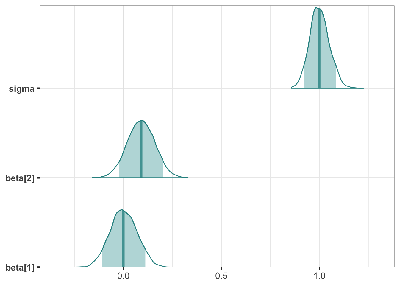
For regression problems, it’s also good to see the regression lines in the posterior distribution. This tells us what kind of lines are compatible with the data and the priors. We use rstan’s extract function to get samples from the posterior.
samples <- as.data.frame(rstan::extract(stan_fit1, pars = c("beta[1]", "beta[2]"))) %>%
  rename(intercept = beta.1., slope = beta.2.) # friendlier variable names

ggplot(samples) +
  geom_abline(aes(intercept = intercept, slope = slope), color = "cadetblue4", alpha = 0.20) +
  geom_abline(aes(intercept = mean(intercept), slope = mean(slope)), color = "black", size = 2) +
  scale_x_continuous(limits = c(-1, 1)) +
  scale_y_continuous(limits = c(-0.45, 0.45)) +
  labs(x = "x",
       y = "y",
       title = "Samples from beta posteriors",
       subtitle = latex2exp::TeX("$N_{samples} = 4000$"))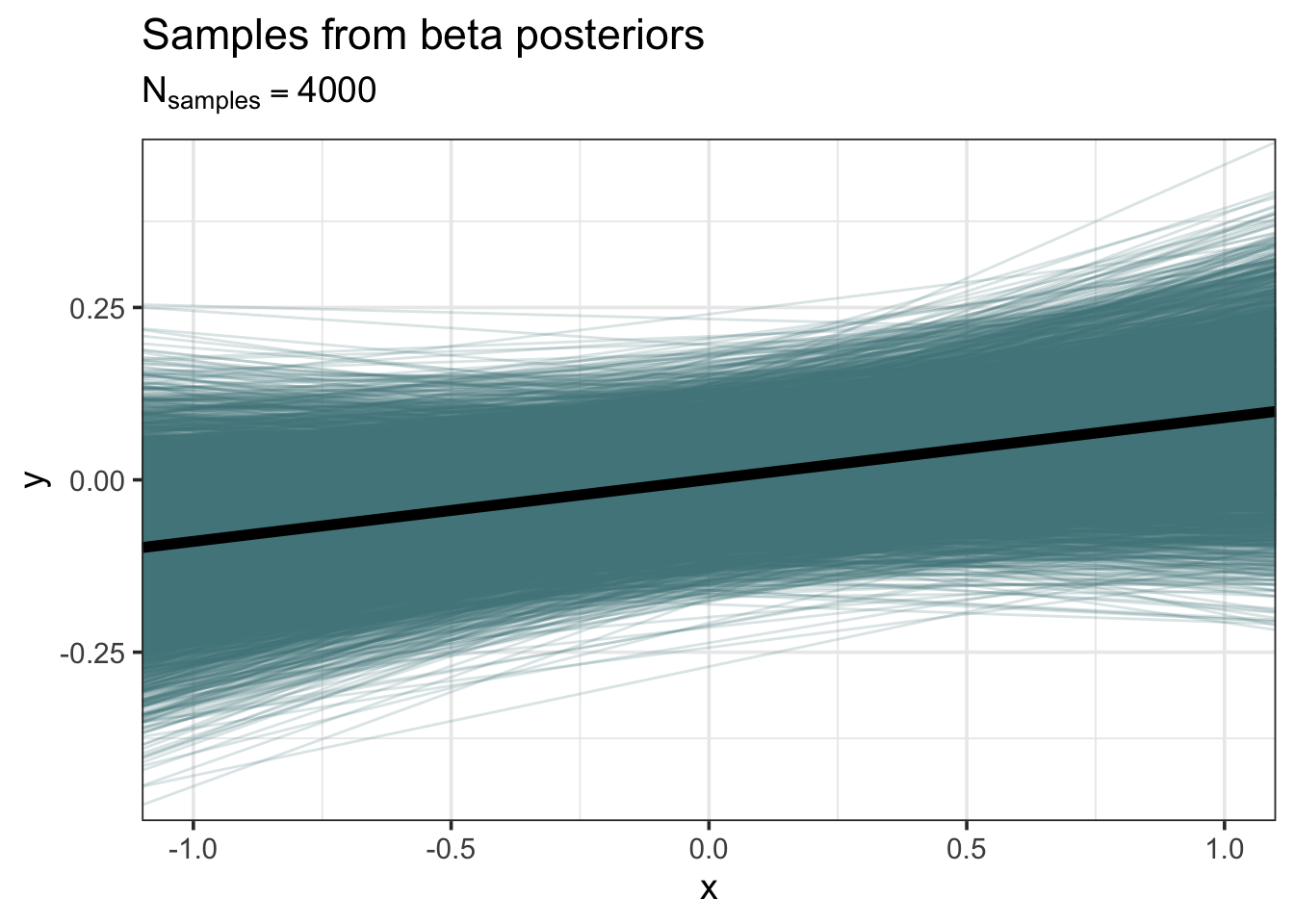
Although the average posterior regression line has positive slope, it’s clear that many lines, even some with negative slope, are compatible.
It doesn’t matter anyway because we know this model is bad - it ignores the clustering. Dealing with the clustering will be the objective for the remainder of this post.
Varying Intercepts and Slopes
Now we’re going to repent for our previous sins and acknowledge that there is shared information among observations of the same participant. What exactly is meant by “shared information”? It means that observations should vary systematically within people as well as across people. The model above makes biased inferences about the effect of x on y because it pools (averages) information greedily.
So our alternative is to assign each participant their own intercept and slope. But we don’t just want to treat participants as completely independent factors - there should be some common variability across all participants in the sample. So we need to walk a fine balance between pooling all the information and considering each participant as independent. This is where we use regularization. Regularization essentially keeps model parameters from getting too large or too certain. In the case of multilevel models, regularization uses some information from the population-level parameters (e.g., the grand mean) to estimate the cluster-specific parameters (e.g., individual participant intercepts and slopes).
It may help to see the model formula:
\[ \begin{aligned} y_i \sim \text{Normal}(\mu, \sigma) \\ \mu_i = \beta_{0,\text{pid}} + \beta_{1, \text{pid}}x_i\\ \begin{bmatrix} \beta_{0,\text{pid}}\\ \beta_{1, \text{pid}} \end{bmatrix} \sim \text{MVNormal}\bigg( \begin{bmatrix} \beta_0\\ \beta_1 \end{bmatrix} , \Sigma \bigg)\\ \Sigma = \left(\begin{array}{cc} \sigma_{\beta_0}&0\\ 0&\sigma_{\beta_1} \end{array}\right)\Omega \left(\begin{array}{cc} \sigma_{\beta_0}&0\\ 0&\sigma_{\beta_1} \end{array}\right) \\ \beta_0 \sim \text{Normal}(0, 1)\\ \beta_1 \sim \text{Normal}(0, 1)\\ \sigma_{\beta_0} \sim \text{Exponential}(1)\\ \sigma_{\beta_1} \sim \text{Exponential}(1)\\ \sigma \sim \text{Exponential}(1)\\ \Omega \sim \text{LKJcorr(2)} \end{aligned} \]
This is nightmare inducing. I’ll go through this slowly, but just know that it really takes time for this stuff to sink it. Don’t expect it to make perfect sense the first (or tenth) time.
The definition of \(\mu\) is thankfully familiar-ish. We now allow each participant (again, denoted by \(\text{pid}\)) to have their own intercept and slope. But think for a moment… these intercepts and slopes don’t just come from nowhere. No, they come from a common distribution of intercepts and slopes. In other words, they come from a multivariate normal distribution!
Aha! So that’s this unpleasant \(\text{MVNormal}\) thing. A multivariate normal distribution takes a vector of mean parameters and a covariance matrix of standard deviations. (Contrast this with the standard normal distribution which takes a single mean parameter and a single SD).
So then what’s this bizarre definition of \(\Sigma\)? We want \(\Sigma\) to be a covariance matrix, but how do we assign a prior to a covariance matrix, which has arbitrary scale and location? The trick is to assign the prior to a correlation matrix instead. This may make intuitive sense to you if you think of a correlation matrix as a standardized version of a covariance matrix. The prior for a correlation matrix is called an LKJ prior (you can see it at the bottom there, \(\text{LKJcorr}\)). Values closer to 1 are less skeptical of strong correlations (-1, +1), whereas higher values (e.g., 2, 4) are more skeptical of strong correlation coefficients.
Ok, so what’s this business with \(\Omega\) sandwiched between these other matrices? These are copies of the same diagonal matrix, containing variances of the \(\beta\) parameters on the diagonal. When you perform this weird-looking matrix multiplication you get a covariance matrix.
What remain are the hyper-priors. This is where the adaptive regularization that I mentioned earlier happens. Take, for example, the prior \(\beta_0 \sim \text{Normal}(0, 1)\). This is the population-level intercept. But note (and this is super important!) that \(\beta_0\) is a multinormal prior for \(\beta_{0, \text{pid}}\). So you can think of it as saying that the individual \(\beta_{0, \text{pid}}\)s come from a common distribution defined by the hyper-prior \(\beta_0\) (and its covariance with \(\beta_1\)). By assigning a prior to \(\beta_0\) we make the model somewhat skeptical of individual intercepts that vary strongly from the average.
You can see similar patterns in the remaining hyper-priors. Now let’s move on to coding the model.
Prior Predictive Simulation
Like we did with the simple linear regression, we should check that my choice of priors is reasonable. I chose conventional priors so we could probably get away without checking them. But it’s good to get into the practice of checking your priors, because there may be times that you have theoretical reasons to choose unconventional priors. Also, prior predictive checking makes it seem like you know what you’re doing and am I’m all for that.
Things unfortunately get more complicated when we simulate data from a varying slopes model. Remember that we’re running the Bayesian inference process in reverse, so we start by simulating hyper-priors and then use those hyper-priors to generate \(\mu\) and \(\sigma\). If you want to run this code yourself, you’ll need to install and load the rethinking package to use rlkjcorr. As of writing, it’s not on CRAN, so you’ll need to install it from GitHub (just uncomment the first couple of lines).
#library(devtools)
#install_github("rmcelreath/rethinking")

beta <- rnorm(2, mean = 0, sd = 1) # b0 and b1
sigma <- rexp(1, 1) # population error
sigma_p <- rexp(2, 1) # sigma0 and sigma1
Omega <- rethinking::rlkjcorr(n = 1, K = 2, eta = 4) # from McElreath's rethinking package

Sigma <- diag(sigma_p) %*% Omega %*% diag(sigma_p)
beta_p <- rmvnorm(N, mean = beta, sigma = Sigma)

x <- matrix(c(rep(1, N * n_days), rnorm(N * n_days, mean = 0, sd = 1)), ncol = 2)
pid <- rep(1:30, each = 7)

sim_dat <- map_dfr(.x = 1:(N * n_days), ~data.frame(
  mu = x[.x, 1] * beta_p[pid[.x], 1] + x[.x, 2] * beta_p[pid[.x], 2],
  pid = pid[.x],
  x = x[.x, 2]
))

sim_dat$y <- rnorm(210, sim_dat$mu, sigma) # creating observed y from mu and sigma

sim_dat <- sim_dat %>%
  mutate(y = real_mean_y + (y * real_sd_y), # unstandardize
         x = real_mean_x + (x * real_sd_x)) # unstandardize
After running this code, you will have an artificial dataset that was generated from one realization of the priors. We want to ensure that our choice of priors is reasonable - that they don’t result in wildly unexpected datasets. So we’ll visualize the scatter of \(x\) and \(y\) variables.
library(gghighlight)

sim_dat %>%
  ggplot(aes(x = x, y = y)) +
  geom_point(size = 3, color = "cadetblue4") +
  gghighlight(pid == 4, use_group_by = FALSE, max_highlight = Inf, use_direct_label = FALSE) +
  labs(title = "Data simulated from priors",
       subtitle = "Green points are from a random participant.\nGrey points are from all other participants.")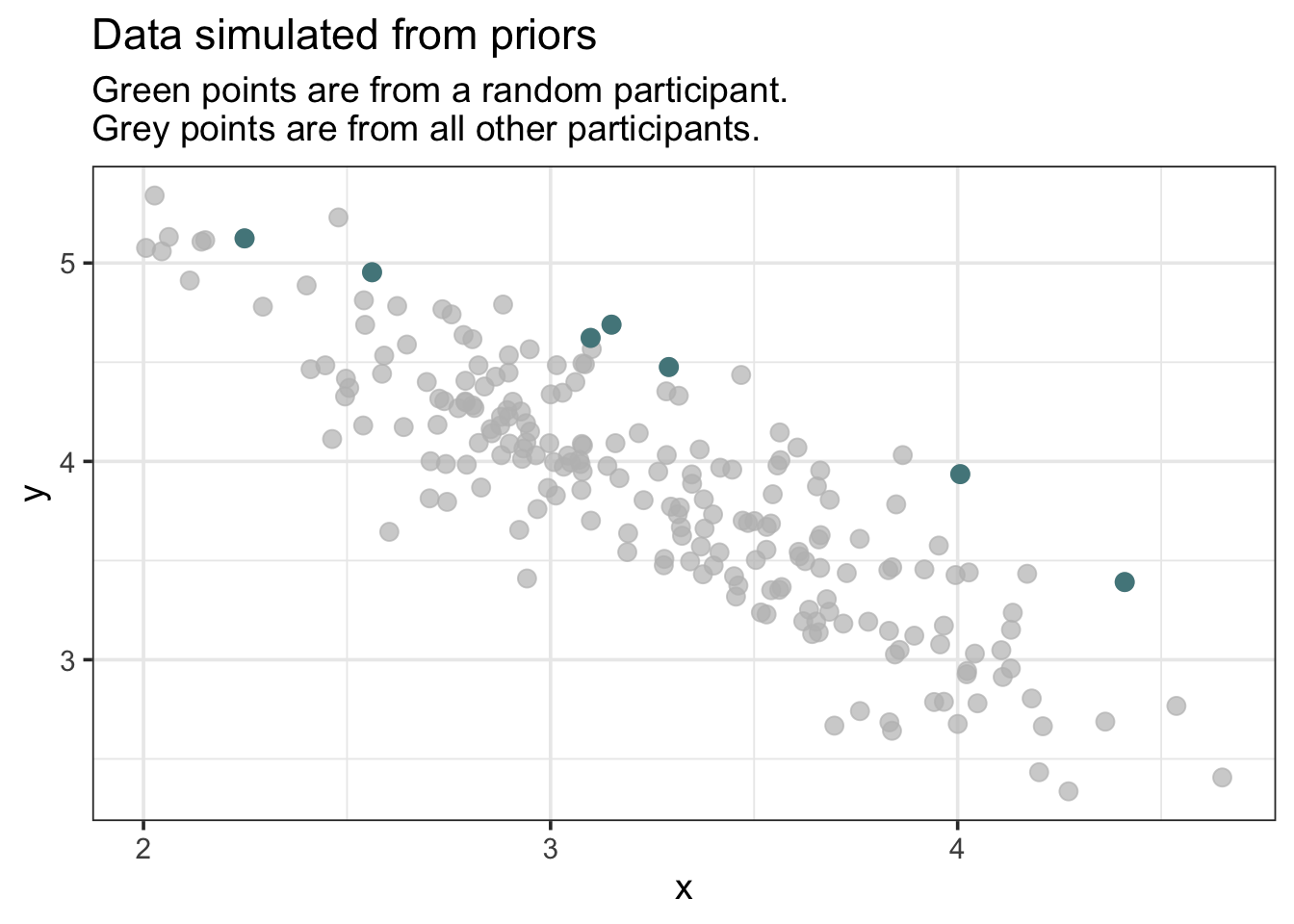
Note that I’ve highlighted one participant. We should see some degree of clustering of the highlighted points, but not always. Rerun the simulation and visualization several times to see how the priors can produce different datasets - some of which seem slightly implausible. If we saw anything truly bizarre, it would be cause to change our priors before analyzing the data for real.
Coding the Model in Stan
We return to Stan to code the model. Now is a good time to revisit the model formula because those characters will make an appearance here. The Stan code can be highly discomforting - I know, I’ve been there (and still am to some degree). But I’ll walk through it slowly.
Data
The data block shouldn’t look too daunting compared to before. What’s new is that we have a number of observations int N_obs and a number of participants int N_pts. We also have a vector of participant ids int pid[N_obs].
// STAN CODE
data {
  int N_obs; // number of observations
  int N_pts; // number of participants
  int K; // number of predictors + intercept
  int pid[N_obs]; // participant id vector
  matrix[N_obs, K] x; // matrix of predictors
  real y[N_obs]; // y vector
}
At first it may seem weird that pid has a length of N_obs; you may wonder why it’s not the length of N_pts. This is because this vector will have the participant identifier for each participant in the dataset. (Look at the column pid in actual data to see what I mean).
Parameters
Plenty different here. We start with vector[K] beta_p[N_pts], which describes a vector of vectors. Specifically, we’re declaring an intercept and slope for each participant (N_pts). We then have vector<lower=0>[K] sigma_p which describes the SD for the participant intercepts and slopes. Now for the hyper-priors, vector[K] beta will hold the means for our intercept and slope hyper-priors and corr_matrix[K] Omega is the \(2 \times 2\) correlation matrix that will be in the multivariate normal prior. Finally, real<lower=0> sigma is the population error that will be in the likelihood of \(y\).
// STAN CODE
parameters {
  vector[K] beta_p[N_pts]; // ind participant intercept and slope coefficients by group
  vector<lower=0>[K] sigma_p; // sd for intercept and slope
  vector[K] beta; // intercept and slope hyper-priors
  corr_matrix[K] Omega; // correlation matrix
  real<lower=0> sigma; // population sigma
}
Model
There are two novelties in this model compared to the simple regression. First, assigning a multivariate normal prior to beta_p, our participant intercepts and slopes, requires some unfamiliar notation. We use the multi_normal command. The first argument is beta because beta is our hyper-prior vector for the mean intercept and slope. What’s this quad_form_diag thing? It is a compact and efficient way of expressing diag(sigma_p) * Omega * diag(sigma_p).
The likelihood looks more or less the same as before. The main difference is that we multiply x by the beta_p parameter. The bracket indexing can be a bit confusing. The expression beta_p[pid[i]] is like saying “the intercept and slope for the \(i^{th}\) participant id”.
// STAN CODE
model {
  vector[N_obs] mu;

  // priors
  beta ~ normal(0, 1);
  Omega ~ lkj_corr(2);
  sigma_p ~ exponential(1);
  sigma ~ exponential(1);
  beta_p ~ multi_normal(beta, quad_form_diag(Omega, sigma_p));

  // likelihood
  for(i in 1:N_obs) {
    mu[i] = x[i] * (beta_p[pid[i]]); // * is matrix multiplication in this context
  }

  y ~ normal(mu, sigma);
}
Full Stan Code
Here is the full Stan code. I’ll save the file as “mod2.stan”.
// STAN CODE
data {
  int N_obs; // number of observations
  int N_pts; // number of participants
  int K; // number of predictors + intercept
  int pid[N_obs]; // participant id vector
  matrix[N_obs, K] x; // matrix of predictors
  real y[N_obs]; // y vector
}

parameters {
  vector[K] beta_p[N_pts]; // ind participant intercept and slope coefficients by group
  vector<lower=0>[K] sigma_p; // sd for intercept and slope
  vector[K] beta; // intercept and slope hyper-priors
  corr_matrix[K] Omega; // correlation matrix
  real<lower=0> sigma; // population sigma
}

model {
  vector[N_obs] mu;

  // priors
  beta ~ normal(0, 1);
  Omega ~ lkj_corr(2);
  sigma_p ~ exponential(1);
  sigma ~ exponential(1);
  beta_p ~ multi_normal(beta, quad_form_diag(Omega, sigma_p));

  // likelihood
  for(i in 1:N_obs) {
    mu[i] = x[i] * (beta_p[pid[i]]); // * is matrix multiplication in this context
  }

  y ~ normal(mu, sigma);
}
Running the Model
Running the model is the same as before. We put the data in a list and point Stan to the model file.
stan_dat2 <- list(
  N_obs = nrow(dat),
  N_pts = max(as.numeric(dat$pid)),
  K = 2, # intercept + slope
  pid = as.numeric(dat$pid),
  x = matrix(c(rep(1, nrow(dat)), (dat$x - mean(dat$x)) / sd(dat$x)), ncol = 2), # z-score for x
  y = (dat$y - mean(dat$y)) / sd(dat$y) # z-score for y
)

stan_fit2 <- stan(file = "mod2.stan",
                  data = stan_dat2,
                  chains = 4, cores = 4)

stan_fit2
## Inference for Stan model: mod2.
## 4 chains, each with iter=2000; warmup=1000; thin=1;
## post-warmup draws per chain=1000, total post-warmup draws=4000.
##
## mean se_mean sd 2.5% 25% 50% 75% 97.5% n_eff Rhat
## beta_p[1,1] 0.00 0.00 0.23 -0.44 -0.15 0.00 0.15 0.43 7192 1
## beta_p[1,2] -0.86 0.00 0.21 -1.27 -1.00 -0.86 -0.71 -0.44 6184 1
## beta_p[2,1] 0.04 0.00 0.21 -0.38 -0.11 0.04 0.18 0.45 6547 1
## beta_p[2,2] -0.31 0.00 0.25 -0.78 -0.47 -0.31 -0.14 0.17 6936 1
## beta_p[3,1] -0.91 0.00 0.22 -1.35 -1.06 -0.92 -0.77 -0.48 5747 1
## beta_p[3,2] 0.58 0.00 0.28 0.01 0.40 0.59 0.77 1.12 6403 1
## beta_p[4,1] -0.19 0.00 0.23 -0.64 -0.34 -0.19 -0.04 0.27 6079 1
## beta_p[4,2] 0.39 0.00 0.19 0.02 0.26 0.39 0.51 0.76 6798 1
## beta_p[5,1] -0.22 0.00 0.22 -0.66 -0.37 -0.22 -0.08 0.23 6051 1
## beta_p[5,2] 0.66 0.00 0.30 0.06 0.46 0.65 0.85 1.25 6424 1
## beta_p[6,1] 0.06 0.00 0.27 -0.46 -0.12 0.07 0.25 0.61 5440 1
## beta_p[6,2] 0.17 0.00 0.36 -0.54 -0.07 0.17 0.41 0.88 5303 1
## beta_p[7,1] 0.28 0.00 0.21 -0.13 0.14 0.28 0.43 0.68 6853 1
## beta_p[7,2] -0.38 0.00 0.18 -0.75 -0.51 -0.38 -0.26 -0.02 7162 1
## beta_p[8,1] 0.84 0.00 0.23 0.38 0.68 0.84 1.00 1.28 5857 1
## beta_p[8,2] -0.25 0.00 0.25 -0.75 -0.42 -0.25 -0.09 0.24 5643 1
## beta_p[9,1] -0.15 0.00 0.21 -0.56 -0.30 -0.15 0.00 0.26 6594 1
## beta_p[9,2] 0.36 0.00 0.22 -0.09 0.21 0.36 0.51 0.80 6256 1
## beta_p[10,1] 0.44 0.00 0.22 0.01 0.30 0.44 0.59 0.87 6533 1
## beta_p[10,2] 0.43 0.00 0.35 -0.25 0.19 0.42 0.65 1.12 6982 1
## beta_p[11,1] 0.80 0.00 0.23 0.35 0.65 0.80 0.96 1.26 5670 1
## beta_p[11,2] -0.27 0.00 0.27 -0.77 -0.45 -0.27 -0.08 0.27 6466 1
## beta_p[12,1] 0.42 0.00 0.22 0.01 0.27 0.42 0.57 0.85 6607 1
## beta_p[12,2] -0.28 0.00 0.19 -0.67 -0.41 -0.27 -0.14 0.10 7727 1
## beta_p[13,1] -0.13 0.00 0.21 -0.55 -0.28 -0.14 0.01 0.28 6268 1
## beta_p[13,2] 0.80 0.00 0.22 0.35 0.65 0.80 0.95 1.23 6691 1
## beta_p[14,1] -0.10 0.00 0.26 -0.61 -0.28 -0.10 0.07 0.39 4745 1
## beta_p[14,2] -0.20 0.00 0.23 -0.65 -0.35 -0.20 -0.04 0.26 5791 1
## beta_p[15,1] -0.39 0.00 0.21 -0.80 -0.54 -0.39 -0.25 0.03 7142 1
## beta_p[15,2] 0.04 0.00 0.18 -0.31 -0.08 0.04 0.17 0.40 7628 1
## beta_p[16,1] 0.70 0.00 0.21 0.28 0.56 0.70 0.85 1.11 6007 1
## beta_p[16,2] 0.05 0.00 0.28 -0.50 -0.14 0.05 0.24 0.59 5859 1
## beta_p[17,1] -0.03 0.00 0.21 -0.46 -0.18 -0.03 0.11 0.38 6024 1
## beta_p[17,2] -0.52 0.00 0.25 -1.04 -0.69 -0.52 -0.36 -0.04 6341 1
## beta_p[18,1] -0.02 0.00 0.21 -0.41 -0.16 -0.03 0.12 0.38 5754 1
## beta_p[18,2] 0.16 0.00 0.19 -0.22 0.03 0.16 0.29 0.54 6008 1
## beta_p[19,1] -0.18 0.00 0.21 -0.57 -0.32 -0.18 -0.04 0.22 6106 1
## beta_p[19,2] 0.28 0.00 0.28 -0.28 0.09 0.28 0.47 0.85 8208 1
## beta_p[20,1] 0.70 0.00 0.21 0.29 0.56 0.70 0.85 1.14 6148 1
## beta_p[20,2] -0.95 0.00 0.28 -1.48 -1.13 -0.95 -0.76 -0.40 6646 1
## beta_p[21,1] -0.88 0.00 0.23 -1.34 -1.03 -0.88 -0.73 -0.44 5747 1
## beta_p[21,2] 0.66 0.00 0.29 0.09 0.47 0.67 0.85 1.23 6673 1
## beta_p[22,1] -0.14 0.00 0.21 -0.55 -0.27 -0.13 0.00 0.26 6794 1
## beta_p[22,2] -0.41 0.00 0.17 -0.74 -0.52 -0.41 -0.30 -0.08 7402 1
## beta_p[23,1] -0.71 0.00 0.21 -1.13 -0.85 -0.70 -0.56 -0.29 6476 1
## beta_p[23,2] 1.48 0.00 0.19 1.10 1.34 1.48 1.61 1.84 6717 1
## beta_p[24,1] -0.02 0.00 0.20 -0.43 -0.16 -0.02 0.11 0.37 6629 1
## beta_p[24,2] 0.57 0.00 0.20 0.19 0.44 0.57 0.70 0.96 6941 1
## beta_p[25,1] 0.39 0.00 0.23 -0.06 0.24 0.39 0.54 0.84 6162 1
## beta_p[25,2] -0.25 0.00 0.24 -0.72 -0.41 -0.25 -0.09 0.22 6687 1
## beta_p[26,1] -0.24 0.00 0.22 -0.68 -0.39 -0.23 -0.08 0.19 7480 1
## beta_p[26,2] 0.00 0.00 0.23 -0.47 -0.15 0.00 0.15 0.46 6449 1
## beta_p[27,1] -0.27 0.00 0.22 -0.69 -0.42 -0.27 -0.12 0.17 5913 1
## beta_p[27,2] -0.18 0.00 0.16 -0.50 -0.29 -0.18 -0.07 0.13 5767 1
## beta_p[28,1] 0.84 0.00 0.22 0.41 0.69 0.84 0.98 1.26 6404 1
## beta_p[28,2] -0.50 0.00 0.21 -0.90 -0.65 -0.50 -0.36 -0.10 7346 1
## beta_p[29,1] -0.03 0.00 0.21 -0.45 -0.17 -0.03 0.12 0.40 6808 1
## beta_p[29,2] 0.56 0.00 0.26 0.04 0.38 0.55 0.74 1.07 6434 1
## beta_p[30,1] -0.19 0.00 0.21 -0.61 -0.33 -0.19 -0.05 0.24 6488 1
## beta_p[30,2] 1.10 0.00 0.28 0.55 0.90 1.09 1.29 1.65 6733 1
## sigma_p[1] 0.53 0.00 0.09 0.38 0.47 0.52 0.58 0.72 4388 1
## sigma_p[2] 0.63 0.00 0.10 0.46 0.56 0.62 0.69 0.85 4487 1
## beta[1] 0.02 0.00 0.10 -0.19 -0.04 0.02 0.09 0.23 5047 1
## beta[2] 0.10 0.00 0.12 -0.14 0.02 0.10 0.18 0.34 5232 1
## Omega[1,1] 1.00 NaN 0.00 1.00 1.00 1.00 1.00 1.00 NaN NaN
## Omega[1,2] -0.45 0.00 0.18 -0.75 -0.58 -0.46 -0.33 -0.07 4125 1
## Omega[2,1] -0.45 0.00 0.18 -0.75 -0.58 -0.46 -0.33 -0.07 4125 1
## Omega[2,2] 1.00 0.00 0.00 1.00 1.00 1.00 1.00 1.00 4165 1
## sigma 0.62 0.00 0.04 0.56 0.60 0.62 0.64 0.69 3513 1
## lp__ 0.02 0.17 6.54 -13.60 -4.06 0.26 4.52 11.79 1411 1
##
## Samples were drawn using NUTS(diag_e) at Sun Mar 21 15:41:38 2021.
## For each parameter, n_eff is a crude measure of effective sample size,
## and Rhat is the potential scale reduction factor on split chains (at
## convergence, Rhat=1).We get a warning about some NA R-hat values and low Effective Samples Size. In this case, these are false alarms - they are merely artifacts of the correlation matrix \(\Omega\) having values that are invariably 1 (like a good correlation matrix should).
mcmc_areas(stan_fit2, pars = c("beta[1]", "beta[2]", "sigma_p[1]", "sigma_p[2]", "sigma"), prob = 0.89) +
  scale_y_discrete(expand = c(0, 0))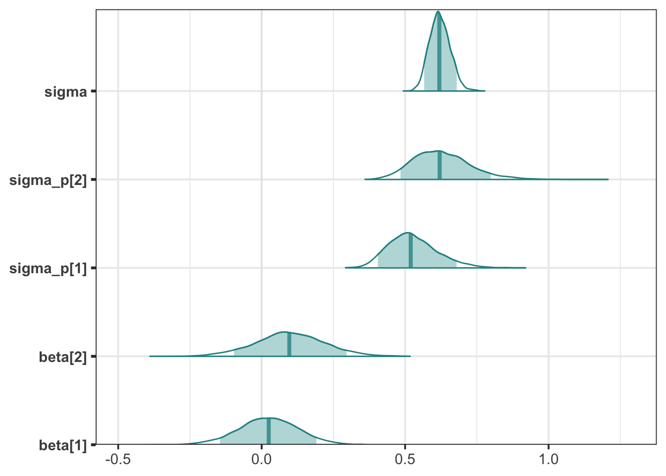
When we look at the posterior densities of some of the parameters. We can see that the overall error, sigma, is lower than in the simple regression. This is because the variance in \(y\) is now shared across population and participant-level error. It’s also worth noting that the model is less certain about the population intercept and slope. The means are roughly the same, but the distribution is more spread out. Because there is participant-level variation in the intercepts and slopes, the model views the population estimates with greater uncertainty.
Visualizing Correlated Slopes and Intercepts
If you look further down the list of parameters in the model output, you’ll see the four \(\Omega\), Omega parameters. These describe the correlation matrix for participant intercepts and slopes. A negative correlation here, tells us that as a participant’s intercept increases, their slope decreases. Let’s plot the participant-specific intercepts and slopes to see this.
We use extract to get the beta_p parameters from the model. Then, using the apply function, we calculate the average of the samples for each beta_p.
beta_p_samples <- rstan::extract(stan_fit2, pars = "beta_p")
beta_p <- as.data.frame(apply(beta_p_samples$beta_p, 2:3, mean)) %>%
  rename(intercept = V1, slope = V2)

beta_p %>%
  ggplot(aes(x = intercept, y = slope)) +
  geom_point(color = "cadetblue4", alpha = 0.75, size = 3) +
  labs(title = "Participant intercept and slope are negatively correlated")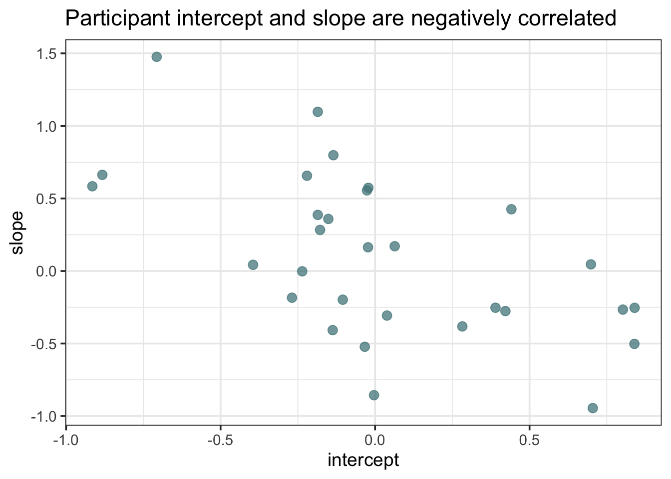
We want to infer beyond the participants in our sample though, so let’s look at the posterior samples for our \(\beta_0\) and \(\beta_1\) parameters. Like with the simple linear regression, we’re going to visualize all the regression lines in the posterior distribution - only now partitioned by intercept. We’ll split the samples into three equal groups based on their intercept. This is of course an arbitrary choice and we’re not implying that there are three distinct groups here. We just want to see how the slope varies by intercept and it’s a lot easier to do this by splitting the samples.
beta_sim <- as.data.frame(rstan::extract(stan_fit2, pars = c("beta[1]", "beta[2]"))) %>%
  rename(intercept = beta.1., slope = beta.2.)

beta_sim %>%
  mutate(int_grp = factor(ntile(intercept, 3), labels = c("[0-33%)", "[33%-66%)", "[66%-100%)"))) %>%
  group_by(int_grp) %>%
  mutate(av_int = mean(intercept),
         av_slope = mean(slope)) %>%
  ungroup() %>%
  ggplot() +
  geom_abline(aes(intercept = intercept, slope = slope), color = "cadetblue4", alpha = 0.20) +
  geom_abline(aes(intercept = av_int, slope = av_slope), color = "black", size = 2) +
  scale_x_continuous(limits = c(-1, 1)) +
  scale_y_continuous(limits = c(-0.75, 0.75)) +
  labs(x = "x",
       y = "y",
       title = "Relation between x and y as a function of intercept.",
       subtitle = "Intercept percentile") +
  facet_wrap(~int_grp) +
  theme(plot.subtitle = element_text(hjust = 0.5))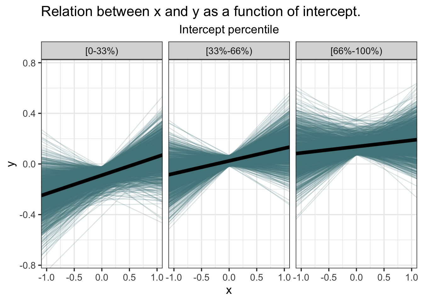
Yes, the slope seems to be getting shallower as the intercept increases.
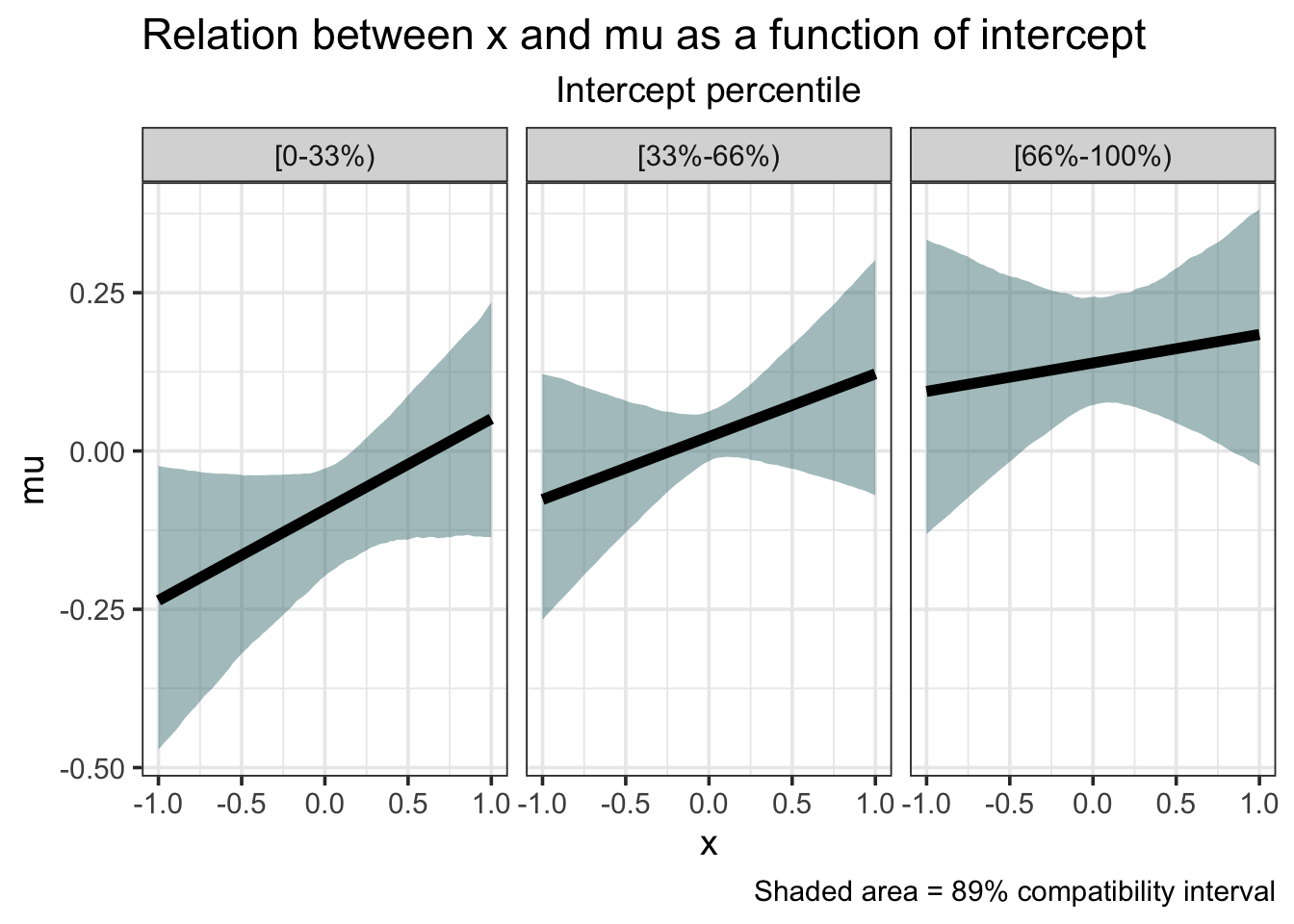
Although I find the ‘many lines’ approach to be appealing, it is more common to present figures displaying means and compatibility intervals (Bayesian equivalent of a confidence interval). We start by creating a sequence of x values over a specified range. Since we’re dealing in standardized units, we’ll make it from -1 to 1. Then for each value of x in this sequence we calculate the expected value of y using the beta samples.
I again make use of dplyr’s map_dfr function to iterate over each value of x and I also bin the intercept into the three groups from before. After this step, we have a large dataframe of 100 x values for each of 4000 samples. Then again for each value of x we calculate the mean (mu) of the samples and its lower and upper bound for the compatiblity interval. Here I adopt McElreath’s convention of 89% compatability interval, but there’s nothing more special about this value than, say, 95%.
seq(-1, 1, length.out = 100) %>% # create a sequence of evenly spaced numbers from -1 to 1
  map_dfr(~ data.frame(y = beta_sim$intercept + .x * beta_sim$slope,
                       x = .x,
                       int = factor(ntile(beta_sim$intercept, 3), levels = c(1, 2, 3),
                                    labels = c("[0-33%)", "[33%-66%)", "[66%-100%)")))) %>%
  group_by(x, int) %>%
  summarise(mu = mean(y),
            lower = quantile(y, probs = 0.055),
            upper = quantile(y, probs = 0.945)) %>%
  ungroup() %>%
  ggplot() +
  geom_ribbon(aes(x = x, ymin = lower, ymax = upper), fill = "cadetblue4", alpha = 0.50) +
  geom_line(aes(x = x, y = mu), color = "black", size = 2) +
  labs(title = "Relation between x and mu as a function of intercept",
       subtitle = "Intercept percentile",
       caption = "Shaded area = 89% compatibility interval") +
  facet_wrap(~int) +
  theme(plot.subtitle = element_text(hjust = 0.5))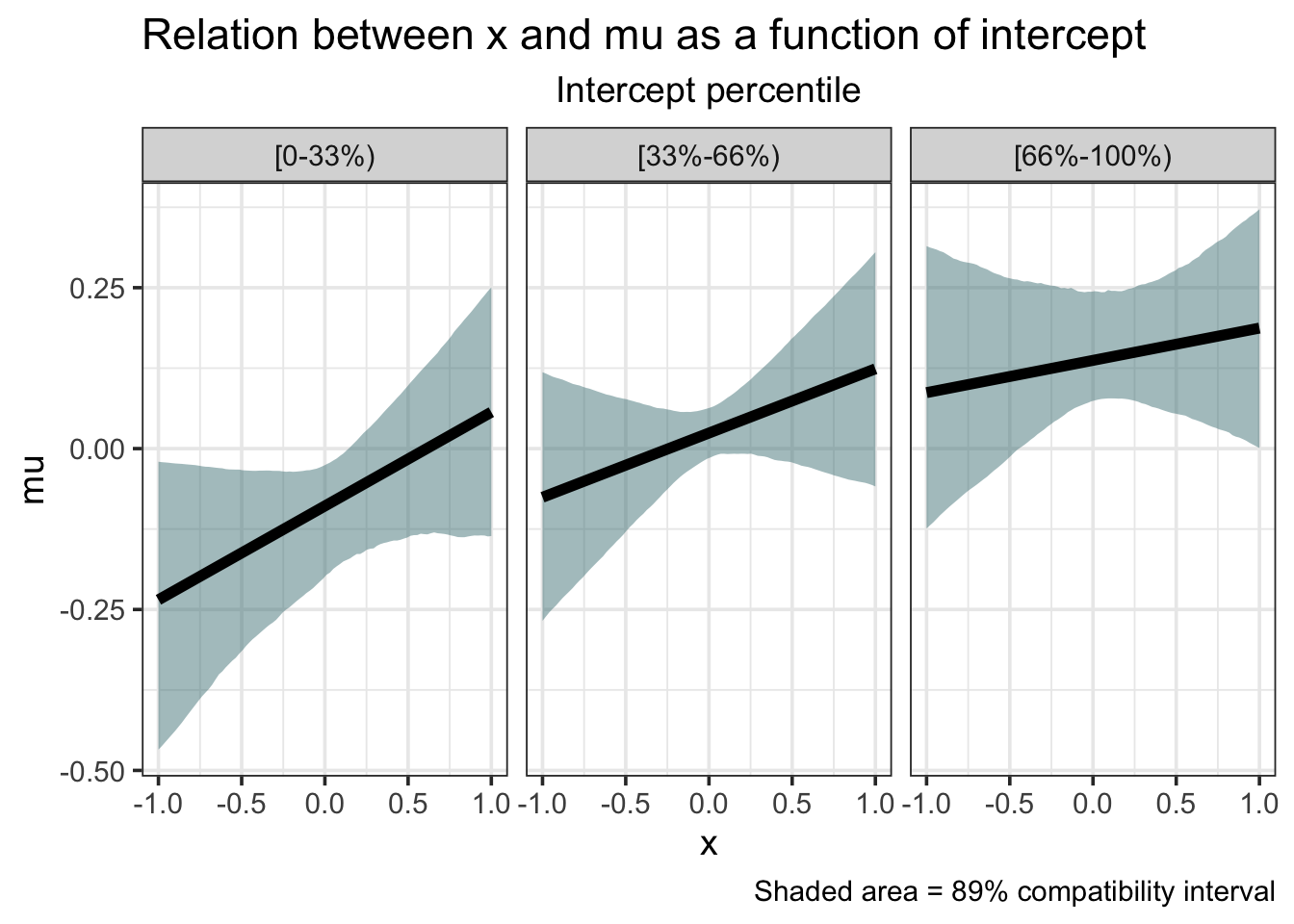
Now that’s a publishable figure!
A More Efficient Varying Slopes Model
Our toy data played nicely with us, but this is rarely the case in the real world. Chances are if you perform the varying slopes model on your own data you’ll encounter efficiency issues and errors. Namely, you’ll be confronted with divergent transitions. These occur when the Hamiltonian Monte Carlo simulation (Stan’s engine) sort of “falls off the track”, so to speak. I won’t elaborate on the math behind divergent transitions (you can find out more here), but I will show how to avoid them by rewriting the model.
You’ll hear people say re-parameterization when they’re talking about this. The more efficient, so-called non-centered parameterization is certainly more efficient, but has some features that initially seem arbitrary. Although the model has different parameters, it is still mathematically the same model. Let’s walk through the Stan code, highlighting the new features.
The data block is the same. In the parameters block we’re going to create a matrix, z_p, that will hold our standardized intercepts and slopes (that’s what the z stands for). The big novelty though is that we’re expressing the correlation matrix as a cholesky_factor_corr. Without going deep into the weeds, a Cholesky factorization of a matrix takes a positive definite matrix (like a correlation matrix) and decomposes it into a product of a lower triangular matrix and its transpose. For linear algebraic reasons, this speeds up the efficiency.
// STAN CODE
data {
  int N_obs; // number of observations
  int N_pts; // number of participants
  int K; // number of predictors + intercept
  int pid[N_obs]; // participant id vector
  matrix[N_obs, K] x; // matrix of predictors
  real y[N_obs]; // y vector
}

parameters {
  matrix[K, N_pts] z_p; // matrix of intercepts and slope
  vector<lower=0>[K] sigma_p; // sd for intercept and slope
  vector[K] beta; // intercept and slope hyper-priors
  cholesky_factor_corr[K] L_p; // Cholesky correlation matrix
  real<lower=0> sigma; // population sigma
}
We have to add a new block called transformed parameters. In this block we can apply transformations to our parameters before calculating the likelihood. What I’m doing here is creating a new matrix of intercepts and slopes called z and then performing some matrix algebra. diag_pre_multiply is an efficient way of doing diag(sigma_p) * L_p.
// STAN CODE
transformed parameters {
  matrix[K, N_pts] z; // non-centered version of beta_p
  z = diag_pre_multiply(sigma_p, L_p) * z_p;
}
For the model block we don’t need to change very much. We use a lkj_corr_cholesky(2) prior for L_p. The likelihood itself is less elegantly expressed than before. Again, the bracket indexing can be confusing. Just remember that z is a matrix where column 1 has the participant intercepts and column 2 has the participant slopes. We still have x as a model matrix but we’re only using the second column, so if we wanted to just have it as a vector in the data that would be fine.
// STAN CODE
model {
  vector[N_obs] mu;

  // priors
  beta ~ normal(0, 1);
  sigma ~ exponential(1);
  sigma_p ~ exponential(1);
  L_p ~ lkj_corr_cholesky(2);
  to_vector(z_p) ~ normal(0, 1);

  // likelihood
  for(i in 1:N_obs) {
    mu[i] = beta[1] + z[1, pid[i]] + (beta[2] + z[2, pid[i]]) * x[i, 2];
  }
  y ~ normal(mu, sigma);
}
Finally, to get back the correlation matrix for the intercepts and slopes, we add one more block to the code: generated quantities. We want to get back Omega, so we use multiply_lower_tri_self_transpose(L_p) to ‘multiply the lower triangular matrix by itself transposed’ (remember what I said about Cholesky factorization).
// STAN CODE
generated quantities {
  matrix[2, 2] Omega;
  Omega = multiply_lower_tri_self_transpose(L_p);
}
Full Stan Code
Here’s the full non-centered parameterization code.
// STAN CODE
data {
  int N_obs; // number of observations
  int N_pts; // number of participants
  int K; // number of predictors + intercept
  int pid[N_obs]; // participant id vector
  matrix[N_obs, K] x; // matrix of predictors
  real y[N_obs]; // y vector
}

parameters {
  matrix[K, N_pts] z_p; // matrix of intercepts and slope
  vector<lower=0>[K] sigma_p; // sd for intercept and slope
  vector[K] beta; // intercept and slope hyper-priors
  cholesky_factor_corr[K] L_p; // Cholesky correlation matrix
  real<lower=0> sigma; // population sigma
}

transformed parameters {
  matrix[K, N_pts] z; // non-centered version of beta_p
  z = diag_pre_multiply(sigma_p, L_p) * z_p;
}

model {
  vector[N_obs] mu;

  // priors
  beta ~ normal(0, 1);
  sigma ~ exponential(1);
  sigma_p ~ exponential(1);
  L_p ~ lkj_corr_cholesky(2);
  to_vector(z_p) ~ normal(0, 1);

  // likelihood
  for(i in 1:N_obs) {
    mu[i] = beta[1] + z[1, pid[i]] + (beta[2] + z[2, pid[i]]) * x[i, 2];
  }
  y ~ normal(mu, sigma);
}

generated quantities {
  matrix[2, 2] Omega;
  Omega = multiply_lower_tri_self_transpose(L_p);
}
I’ll save it to the working directory as “mod2-nc.stan”.
Running the Model
Running the model is the same as before. The data is exactly the same, but for symmetry I’ve renamed it stan_dat3.
stan_dat3 <- list(
  N_obs = nrow(dat),
  N_pts = max(as.numeric(dat$pid)),
  K = 2, # intercept + slope
  pid = as.numeric(dat$pid),
  x = matrix(c(rep(1, nrow(dat)), (dat$x - mean(dat$x)) / sd(dat$x)), ncol = 2), # z-score for x
  y = (dat$y - mean(dat$y)) / sd(dat$y) # z-score for y
)

stan_fit3 <- stan(file = "mod2-nc.stan",
                  data = stan_dat3,
                  chains = 4, cores = 4)

stan_fit3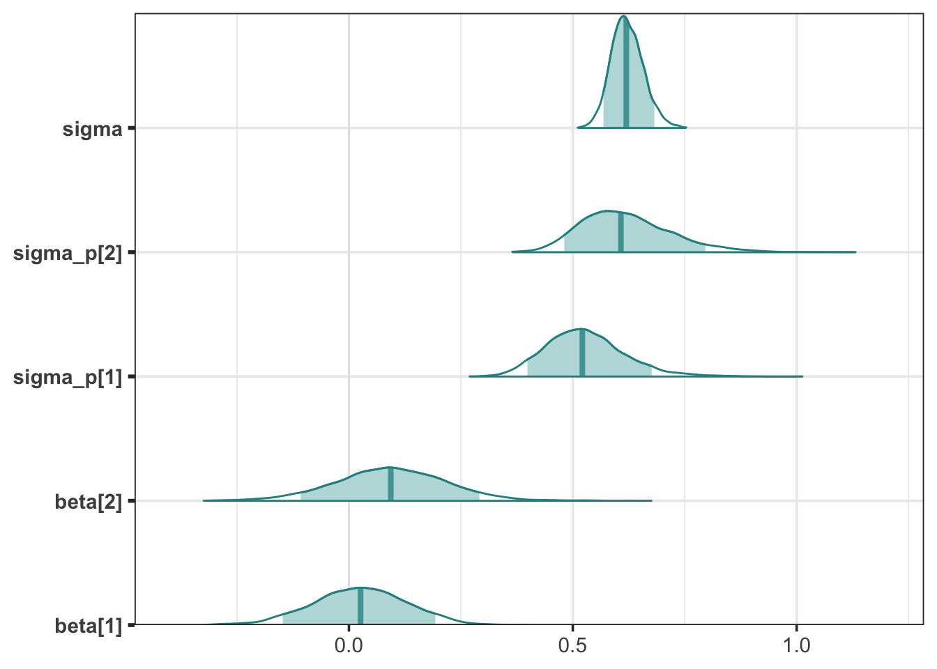
Looking at the posterior densities for the population betas, sigma, and participant sigmas, they are same as the previous model with only minor differences in sampling error.
In summary, use the non-centered parameterization (the one with the Cholesky factorization) when you find your varying effects models misbehaving.
Resources
I couldn’t end this post without recommending Richard McElreath’s Statistical Rethinking. It is a bastion of Bayesian knowledge and truly a joy to read. There are also several blog posts that I recommend if you’re looking for more multilevel Stan fun: