A first look at torch for R
In this post, I explore torch - a package for R that mirrors the PyTorch framework for deep learning.
Motivation
I’ve been a bit reluctant to join in on the deep learning hype for some time. Much of this I attribute to my lack of enthusiasm toward Python frameworks for deep learning. Don’t get me wrong. Tensorflow + Keras offers an intuitive API for neural nets, but can I just be frank and say I like R better for everything else?
A few years back, I was briefly tantalized by the tensorflow package for R, but I couldn’t establish a solid workflow with its Python backend constantly getting in the way. (Many an enfuriating hour was spent fruitlessly trying to configure my GPU).
Jump ahead to autumn of 2020 and the torch package for R is announced. My enthusiasm is rekindled when I hear that torch is a native R package that uses a C++ backend instead of Python. The clouds began to part.
However, torch is still somewhat in its infancy and although it is capable of what most mature deep learning frameworks can do, it doesn’t offer the kind of high-level API that makes it intuitive to grasp for beginners. The purpose of this post is to help the reader get familiar with the torch package. This post will be focused more on the programming aspects of torch rather than the mathematical and theoretical aspects of deep learning.
Road Map
This post will be broken into 4 steps:
- Get and explore the data
- Create a
Datasetobject - Build a network
- Run the model
1. Get and explore the data
In this tutorial, we’ll use the Star Type Classification Data from NASA shared on Kaggle.com. The data contains details about stars and their type, which we will attempt to predict.
I like to use pins to import data directly from Kaggle into R. The code below will show how to get the data using pins, assuming you have an account with Kaggle. You can also just go to the link and download the data as a .csv if you prefer.
library(tidyverse)
library(pins)

# --- RUN FIRST IF YOU HAVEN'T USED KAGGLE AND PINS BEFORE
# If you have an account you can get your token at https://www.kaggle.com/me/account
# and download your .json token.

# board_register_kaggle(token = "path/to/kaggle.json")
# ---

pin_name <- pin_find("star-type-classification", board = "kaggle")[[1]]

pin_dir <- pin_get(pin_name, board = "kaggle")

stars_raw <- read_csv(pin_dir)

head(stars_raw)
## # A tibble: 6 x 7
## Temperature L R A_M Color Spectral_Class Type
## <dbl> <dbl> <dbl> <dbl> <chr> <chr> <dbl>
## 1 3068 0.00240 0.17 16.1 Red M 0
## 2 3042 0.0005 0.154 16.6 Red M 0
## 3 2600 0.000300 0.102 18.7 Red M 0
## 4 2800 0.0002 0.16 16.6 Red M 0
## 5 1939 0.000138 0.103 20.1 Red M 0
## 6 2840 0.00065 0.11 17.0 Red M 0The data includes the following features to use as predictors:
L= Relative Luminosity (L/Lo)R= Relative Radius (R/Ro)A_M= Absolute MagnitudeTemperature= Temperature in KelvinColor= Star colorSpectral_Class
We want to use these to predict star type, which is encoded in the Type variable. There are six different types of stars: 0 = Red Dwarf, 1 = Brown Dwarf, 2 = White Dwarf, 3 = Main Sequence, 4 = Super Giants, and 5 = Hyper Giants.
There are some categorical features here. Color is one we’ll take a closer look at.
stars_raw %>%
  count(Color, sort = TRUE)
## # A tibble: 17 x 2
## Color n
## <chr> <int>
## 1 Red 112
## 2 Blue 56
## 3 Blue-white 26
## 4 Blue White 10
## 5 yellow-white 8
## 6 White 7
## 7 Blue white 4
## 8 white 3
## 9 Yellowish White 3
## 10 Orange 2
## 11 Whitish 2
## 12 yellowish 2
## 13 Blue-White 1
## 14 Orange-Red 1
## 15 Pale yellow orange 1
## 16 White-Yellow 1
## 17 Yellowish 1Lots of red and blue - that’s ok. But what’s the deal with different categories for Blue-white and Blue White? We see a similar pattern elsewhere. We’d do well to implement some string handling as well as factor lumping. For this, we’ll leverage the stringr and forcats packages, respectively, which are loaded as part of the tidyverse.
Instead of directly changing the data, I’m going to create a function that we can include in a preprocessing pipeline.
fix_color <- function(x, n = 5) {
  x_lower <- str_to_lower(x)
  x_fix <- str_replace(x_lower, " |-", "_") # replaces either blank space or '-' with '_'
  x_lump <- fct_lump(x_fix, n, other_level = "other")
  x_lump
}

# Test
stars_raw %>%
  mutate(Color = fix_color(Color)) %>%
  count(Color, sort = TRUE)
## # A tibble: 6 x 2
## Color n
## <fct> <int>
## 1 red 112
## 2 blue 56
## 3 blue_white 41
## 4 other 13
## 5 white 10
## 6 yellow_white 82. torch Datasets
Before we dig into the code we should familiarize ourselves with some torch semantics.
Tensors
If you know a little about deep learning, you know that it works with tensors. A tensor is like a matrix but it can have more dimensions. As well, tensors can be on a GPU which makes for much faster learning.
In torch, our data must be represented as a torch_tensor object. torch provides a number of functions for creating tensors from scratch or transforming native R objects to tensors and back:
library(torch)

# --- First time using torch? Run this once:
# install_torch()
# ---

# Create 2 X 3 tensor of random numbers
torch_rand(2, 3)
## torch_tensor
## 0.3814 0.0616 0.8063
## 0.6118 0.6273 0.3036
## [ CPUFloatType{2,3} ]# Create tensor from R matrix
mat <- matrix(c(1, 4, 7,
2, 5, 2), nrow = 2, byrow = TRUE)
my_tensor <- torch_tensor(mat)
my_tensor## torch_tensor
## 1 4 7
## 2 5 2
## [ CPUFloatType{2,3} ]# Convert back to R object
as_array(my_tensor)## [,1] [,2] [,3]
## [1,] 1 4 7
## [2,] 2 5 2Datasets
In torch, a Dataset is kind of like a traditional data.frame, but it has a few special features that make it easier for deep learning. Instead of thinking of it as a static spreadsheet, think of it as a function that will feed data into our network in bite-sized chunks or batches.
We create a Dataset object using the dataset function. It’s essentially a list of attributes and methods that we can access from the Dataset. A Dataset should have the following attributes:
Name (e.g.,
"stars_dataset")initializemethod that takes in adata.frame.getitemmethod that allows us to index the Dataset (e.g.,stars_dataset[1]to get first row of data).lengthmethod to get the number of rows in the Dataset.
It’s also in here that we run our preprocessing on the data and convert everything to a torch_tensor. Moreover, it’s wise to split our predictors into separate tensors for numeric and categorical types because we’ll treat these differently in our neural net.
stars_dataset <- dataset(

  name = "stars_dataset",

  initialize = function(df) {

    # Data preprocessing
    stars_pp <- df %>%
      select(-Type) %>%
      mutate(across(c("Temperature", "L", "R"), log10),
             Color = fix_color(Color))

    # Numeric predictors
    self$x_num <- stars_pp %>%
      select(where(is.numeric)) %>%
      as.matrix() %>%
      torch_tensor()

    # Categorical predictors
    self$x_cat <- stars_pp %>%
      select(!where(is.numeric)) %>%
      mutate(across(everything(), ~as.integer(as.factor(.x)))) %>%
      as.matrix() %>%
      torch_tensor()

    # Target data
    type <- as.integer(df$Type) + 1
    self$y <- torch_tensor(type)
  },

  .getitem = function(i) {
    x_num <- self$x_num[i, ]
    x_cat <- self$x_cat[i, ]
    y <- self$y[i]

    list(x = list(x_num, x_cat),
         y = y)
  },

  .length = function() {
    self$y$size()[[1]]
  }
)
Aside: torch and R6 Classes
A lot of the things we make in torch - Datasets, modules, networks - take the form of an R6 class structure. What is R6? R6 is a framework for object-oriented programming in R. You may be unfamiliar with R6 and that’s fine.
The biggest stumbling block I encountered with R6 was understanding what self is and where it comes from. I like to think of self as a list where we can store things like data or functions. For example, a Dataset object has tensors and we can make those tensors part of the Dataset by assigning them to self. self is automatically built in to every R6 class, so you don’t have to create it yourself.
If you want a deeper dive into R6 Classes, check out the chapter on R6 in Hadley Wickham’s Advanced R.
End Aside
We need to instantiate our Dataset. As is typical in machine learning, we’ll create a training data set and another data set for evaluation. Because our data is small, we’ll just stick with training and validation sets. If we had more data, we’d create a test data set for final model evaluation.
set.seed(941843)

length_ds <- length(stars_dataset(stars_raw))

train_id <- sample(1:length_ds, ceiling(0.80 * length_ds))
valid_id <- setdiff(1:length_ds, train_id)

# Datasets
train_ds <- stars_dataset(stars_raw[train_id, ])
valid_ds <- stars_dataset(stars_raw[valid_id, ])
Dataloaders
We have our training and validation Datasets. Last thing we need to do with the data is create dataloader objects. A dataloader feeds batches of data through the network. We shuffle the training set so that at every epoch (iteration of the learning phase) the data is reshuffled.
# Dataloaders
train_dl <- train_ds %>%
  dataloader(batch_size = 25, shuffle = TRUE)

valid_dl <- valid_ds %>%
  dataloader(batch_size = 25, shuffle = FALSE)
3. Building the neural net
With the data spoken for we can move on to creating the neural net architecture. torch represents network architectures as one or more modules. As we’ll see, modules can be combined together to make more complex models out of separate, reusable chunks. We’ll start this section by creating a small module to handle the categorical features in the data and then a larger module representing our full neural net.
Embedding Categorical Features
Our data has two categorical features, Color and Spectral Class. Because these features don’t have an inherent ordering to them, we can’t use the raw numeric values. The solution is to use embeddings. This means we represent each level of the categorical feature in some n-dimensional space. The space is represented by a trainable vector. In other words, the embeddings are parameters in the model.
We use nn_module to create the embedding layer. In torch, nn_modules have a forward method. The forward method details how the module will feed data through the network when the network is making predictions (i.e., feed-forward). This also means that the nn_module contains parameters that can learn.
# Borrows quite a lot from https://blogs.rstudio.com/ai/posts/2020-11-03-torch-tabular/
embedding_mod <- nn_module(

  initialize = function(levels) {

    self$embedding_modules = nn_module_list(
      map(levels, ~nn_embedding(.x, embedding_dim = ceiling(.x/2)))
    )
  },

  forward = function(x) {

    embedded <- vector("list", length(self$embedding_modules))
    for(i in 1:length(self$embedding_modules)) {
      # gets the i-th embedding module and calls the function on the i-th column
      # of the tensor x
      embedded[[i]] <- self$embedding_modules[[i]](x[, i])
    }

    torch_cat(embedded, dim = 2)
  }
)
There’s a lot going on here. Taking it piece by piece, we create a list called embedding_modules using the nn_module_list function. For each set of levels (there are two sets because there are two categorical features) we instantiate an embedding layer - nn_embedding with dimension roughly half the number of levels.
The forward piece is responsible for taking each of the embedding layers and using it on each of the categorical predictors. torch_cat then combines everything together into one tensor along the second dimension.
Neural net architecture
Our neural net will consist of a series of layers and activation functions. In the initialize method we create the layers. Because we’re dealing with fairly simple tabular data, we’ll stick with fully-connected layers (customarily denoted as fc).
I follow the advice in the torch for tabular blog post and use the number of levels + the number of numeric columns as the first input layer dimension. For a fully-connected network, the number of features we input in each layer should equal the number of features outputted by the preceding layer.
In the forward method, we pass the predictors through each layer in the network. Note that we output with a softmax activation function because we are predicting a categorical variable with more than two possible values.
net <- nn_module(

  "stars_net",

  initialize = function(levels, n_num_col) {

    self$embedder <- embedding_mod(levels)

    # calculate dimensionality of first fully-connected layer
    embedding_dims <- sum(ceiling(levels / 2))

    self$fc1 <- nn_linear(in_features = embedding_dims + n_num_col,
                          out_features = 32)
    self$fc2 <- nn_linear(in_features = 32,
                          out_features = 16)
    self$output <- nn_linear(in_features = 16,
                             out_features = 6) # number of Types
  },

  forward = function(x_num, x_cat) {

    embedded <- self$embedder(x_cat)

    predictors <- torch_cat(list(x_num$to(dtype = torch_float()), embedded), dim = 2)

    predictors %>%
      self$fc1() %>%
      nnf_relu() %>%
      self$fc2() %>%
      nnf_relu() %>%
      self$output() %>%
      nnf_softmax(2) # along 2nd dimension (i.e., rowwise)
  }
)
Ok, so we have defined the network, but we still need to instantiate it. Our net needs a vector of levels and the number of numeric features.
levels <- stars_raw %>%
  mutate(Color = fix_color(Color)) %>%
  select(!where(is.numeric)) %>%
  map_dbl(n_distinct) %>%
  unname()

n_num_col <- ncol(train_ds$x_num)
The network can run on a GPU if you have one, otherwise a CPU is fine. (For this example the model will run fast enough on CPU anyway).
# Use GPU if available, otherwise CPU
device <- if(cuda_is_available()) {
  torch_device("cuda:0")
} else {
  "cpu"
}

model <- net(levels, n_num_col)

model <- model$to(device = device)
4. Run the model
To run the model we need to choose an optimizer. This is the algorithm that will modify the weights so as to minimize the loss function. I’ll use optim_asgd but you can experiment with others like optim_sgd.
We also need to set up the training and evaluation loop. This part looks a bit daunting, but a lot of it is repetition (we do almost the same thing for both the training and evaluation). Perhaps the most awkward part is where we assign the output. Ignore the to$device = device) part and just look at the subscripted pieces, b$x[[1]] and b$x[[2]]. We’re just passing in the numeric and categorical features, respectively. The model uses the weights to make a prediction.
Once we have a prediction, which we assign to output, we need to compute the loss. For multilabel classification, we use nnf_cross_entropy, passing it the output and the true label. The rest is boilerplate to backpropagate and the loss and update the weights.
torch_manual_seed(414412)
optimizer <- optim_asgd(model$parameters, lr = 0.025)
n_epochs <- 140

for(epoch in 1:n_epochs) {

  # set the model to train
  model$train()

  train_losses <- c()

  # Make prediction, get loss, backpropagate, update weights
  coro::loop(for (b in train_dl) {
    optimizer$zero_grad()
    output <- model(b$x[[1]]$to(device = device), b$x[[2]]$to(device = device))
    loss <- nnf_cross_entropy(output, b$y$to(dtype = torch_long(), device = device))
    loss$backward()
    optimizer$step()
    train_losses <- c(train_losses, loss$item())
  })

  # Evaluate
  model$eval()

  valid_losses <- c()
  valid_accuracies <- c()

  coro::loop(for (b in valid_dl) {
    output <- model(b$x[[1]]$to(device = device), b$x[[2]]$to(device = device))
    loss <- nnf_cross_entropy(output, b$y$to(dtype = torch_long(), device = device))
    valid_losses <- c(valid_losses, loss$item())
    pred <- torch_max(output, dim = 2)[[2]]
    correct <- (pred == b$y)$sum()$item()
    valid_accuracies <- c(valid_accuracies, correct/length(b$y))
  })

  if(epoch %% 10 == 0) {
      cat(sprintf("Epoch %d: train loss: %3f, valid loss: %3f, valid accuracy: %3f\n",
                  epoch, mean(train_losses), mean(valid_losses), mean(valid_accuracies)))
  }
}
## Epoch 10: train loss: 1.692698, valid loss: 1.647046, valid accuracy: 0.564348
## Epoch 20: train loss: 1.623896, valid loss: 1.560694, valid accuracy: 0.544348
## Epoch 30: train loss: 1.577717, valid loss: 1.530740, valid accuracy: 0.627826
## Epoch 40: train loss: 1.519202, valid loss: 1.459082, valid accuracy: 0.667826
## Epoch 50: train loss: 1.461917, valid loss: 1.413592, valid accuracy: 0.687826
## Epoch 60: train loss: 1.422795, valid loss: 1.376273, valid accuracy: 0.687826
## Epoch 70: train loss: 1.393934, valid loss: 1.346061, valid accuracy: 0.689565
## Epoch 80: train loss: 1.350427, valid loss: 1.309352, valid accuracy: 0.791304
## Epoch 90: train loss: 1.322084, valid loss: 1.277471, valid accuracy: 0.793043
## Epoch 100: train loss: 1.280443, valid loss: 1.256384, valid accuracy: 0.793043
## Epoch 110: train loss: 1.254480, valid loss: 1.237143, valid accuracy: 0.813043
## Epoch 120: train loss: 1.231149, valid loss: 1.216946, valid accuracy: 0.894783
## Epoch 130: train loss: 1.216650, valid loss: 1.203064, valid accuracy: 0.894783
## Epoch 140: train loss: 1.201882, valid loss: 1.189315, valid accuracy: 0.936522We can understand better how the model performs with a confusion matrix.
library(yardstick)
pred <- torch_max(model(valid_ds$x_num, valid_ds$x_cat), dim = 2)[[2]] %>%
as_array()
truth <- valid_ds$y %>%
as_array()
type_levels <- c("Red Dwarf", "Brown Dwarf", "White Dwarf",
"Main Sequence", "Super Giant", "Hyper Giant")
confusion <- bind_cols(pred = pred, truth = truth) %>%
mutate(across(everything(), ~factor(.x, levels = 1:6, labels = type_levels))) %>%
conf_mat(truth, pred)
autoplot(confusion, type = "heatmap") +
scale_fill_distiller(palette = 2, direction = "reverse")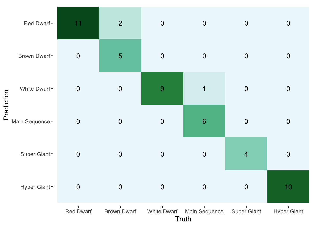 In the end, it’s the small amount of data that keeps us from doing much more with this model. We could probably do just as well with multinomial regression. Still, the goal was to explore
 torch on a fairly tame data set.
Concluding Remarks
So is it worth it for R users to learn torch? Although the torch package has all the necessary functionality for building sophisticated deep learning models, I think it still poses challenges, particularly for new users. The syntax is jarring for those unfamiliar with R6 and it lacks a high-level API geared toward those who want to build models quickly. Online documentation is also somewhat sparse compared to more mature frameworks with PyTorch and Tensorflow.
All of these issues are likely to be resolved as torch matures and the community grows. For now, I’m just thrilled to have such a powerful, native R deep learning framework, and I’m excited to see what the future has in store for torch!
Resources
I’m extremely grateful for the torch documentation and tutorials for helping me get started with this post. I’m also indebted to the brilliant blog posts on the RStudio AI Blog. In particular, I leaned heavily on this post by Sigrid Keydana for insights as well as for help with the embedding module.